DM828 - Introduction to Artificial Intelligence
Exercise Sheet 4, Autumn 2011 [pdf format]

Prepare the following exercises for discussion in class on Thursday, December 1.

Exercises

1. Exercise 18.4, 18.5, 18.10, 18.29
2. In a classification task you are given the following data points: Negative: (-1, -1) (2, 1) (2, -1); Positive: (-2, 1) (-1, 1) (1,-1). The points are depicted in Figure 1.

   ---

   

   Figure 1: The data points for classification.

   ---

   Decision Tree

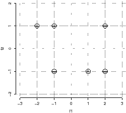
   1. Construct a decision tree using the recursive bi-partitioning algorithm based on information gain described in class. (Discretize the continue scale considering for f₁ only the values {−1.5,0,1.5} and for f₂ only 0.) Represent graphically the tree constructed and draw the decision boundaries in the Figure 1.
   2. Explain how you chose the top-level attribute in the tree. Table 1 might be useful.

      ---

      x	y	−(x/y) · log(x/y)	x	y	−(x/y) · log(x/y)
      1	2	0.50	1	5	0.46
      1	3	0.53	2	5	0.53
      2	3	0.39	3	5	0.44
      1	4	0.50	4	5	0.26
      3	4	0.31

      Table 1: Numerical values for the computation of information gains.

      ---

   3. Apply χ² pruning.
   4. Use the tree to predict the outcome for the new point (1,1).

   Nearest Neighbor

   1. Draw the decision boundaries for 1-Nearest Neighbors on the Figure 1. Make it accurate enough so that it is possible to tell whether the integer-valued coordinate points in the diagram are on the boundary or, if not, which region they are in.
   2. What class does 1-NN predict for the new point: (1, 1) Explain why.
   3. What class does 3-NN predict for the new point: (1, 0) Explain why.
   4. In general, how would you select between two alternative values of k for use in k-nearest neighbors?

   Perceptron

   1. Imagine to apply the perceptron learning algorithm to the points in Figure 1. Describe qualitatively what the result would be.
3. Consider neural networks with inputs in the range [0,1] and with a step function g. A network is defined by the weights on the links and a threshold value of g at each node.
   • (a) In Boolean logic, the majority function is a function from n inputs to one output. The value of the operation is false when n/2 or more arguments are false, and true otherwise. Draw a network that represent the majority function for 4 input nodes.
   • (b) Draw a network that represent the “exactly two out of three” function for three inputs.
   • (c) Draw a network to simulate the XOR operator in Boolean logic. XOR (exclusive-or) is a logical operator that results in the output being true if one of the inputs, but not both, is true. If both inputs are true the output is false.
4. Using R do exercise 18.24. The commands you may try are nnet from package nnet, rpart from package rpart, knn from package class, the glm function (check example in ?predict.glm). Look at the examples of these methods by ?function. nnet uses one hidden layer. To implement the single layer perceptron you may try to use the following lines for stochastic gradient descent with the needed changes:

   sigma <- function(w,point) { x <- c(point,1) sign(w %*% x) } w.0 <- c(runif(1),runif(1),runif(1)) w.t <- w.0 for (j in 1:1000) { i <-sample(1:50,1) # or (j-1)%%50 + 1 diff <- y[i,3] - sigma(w.t, c(x[i,1],x[i,2])) w.t <- w.t+0.2*diff * c(x[i,1],x[i,2],1) }

   Test also the batch version of gradient descent.

   More data to analyse are available at UCI Machine Learning Repository.