DM828 - Introduction to Artificial Intelligence Exercise Sheet 7, Autumn 2011 [pdf format]

Exercises

Search

Suppose you have two containers, initially empty. One has a capacity of exactly 3 liters; the other has a capacity of 5 liters. You can pour water from one container to another, empty a container, or fill a container at any time. Your problem is to place exactly 4 liters of water in the 5-liter container. Describe how this problem could be framed as a search problem defining the related components. Solve the problem within this framework and report the search performed.

Prove that the set of states expanded by algorithm A^* is a subset of those expanded by breadth-first search.

Every day that he leaves work, Albert the Absent-minded Professor, toggles his light switch according to the following protocol: (i) if the light is on, he switches it off with probability 0.80; and (ii) if the light is off, he switches it on with probability 0.30. At no other time (other than the end of each day) is the light switch touched.

[a)]Suppose that on Monday night, Albert’s office is equally likely to be light or dark. What is the probability that his office will be lit all the other four nights of the week (Tuesday through Friday)?
Suppose that you observe that his office is lit on both Monday and Friday nights. Compute the expected number of nights, from that Monday through Friday, that his office is lit.

Now suppose that Albert has been working for five years (i.e., assume that the Markov chain is in steady state).

Is his light more likely to be on or off at the end of a given workday?

Consider a variant of the game Nim. A number of tokens are placed on a table between the two opponents; at each move, the player must divide a pile of tokens into two nonempty piles of different sizes. Thus, 6 tokens may be divided into piles of 5 and 1 or 4 and 2, but not 3 and 3. The first player who can no longer make a move losses the game. Explore exhaustively the search space for a number of tokens equal to 7 and represent the game tree. Who will win the game?

Design a spam mail classifier by means of k-nearest neighbor and decision trees and report your design choices. What is a lazy classifer and which of the two methods mentioned is such?

Suppose that a fair-looking coin is tossed three times and lands heads each time. Show that a classical maximum likelihood estimate of the probability of landing heads would give 1, implying that all future tosses will land heads. By contrast, show that a Bayesian approach with a prior of 0.5 for the probability of heads would lead to a much less extreme conclusion on the posterior probability of observing heads.

Bayesian Networks and Learning

Consider a Naive Bayes problem with three features, x₁, x₂, x₃. Imagine that we have seen a total of 16 training examples, 8 positive (with y = 1) and 8 negative (with y = 0). In Table 1 you find some of the counts.

y = 0 y = 1

x₁ = 1 7 7

x₂ = 1 1 1

x₃ = 1 3 5

Table 1: Count table

What are the values estimated from the data for the following parameters:

Pr(x₁ = 1|y = 0)=θ₁₀,
Pr(x₂ = 1|y = 1)=θ₂₁,
Pr(x₃ = 0|y = 0)=1−θ₃₀?

(You need to show the full derivation, answers by intuition without analytical justification do not count.)

Bayesian Networks – Inference.

Figure 1 shows a graphical model with conditional probabilities tables about whether or not you will panic at an exam based on whether or not the course was boring (“B”), which was the key factor you used to decide whether or not to attend lectures (“A”) and revise doing the exercises after each lecture (“R”).

[ place/.style=ellipse,draw=black!50,fill=black!20,thick, inner sep=0pt,minimum size=1cm, pre/.style=<-,shorten <=1pt,>=angle 60,semithick, post/.style=->,shorten >=1pt,>=stealth’,semithick, transition/.style=rectangle,draw=black!100,fill=black!20,thick, inner sep=0pt,minimum size=3mm] [place] (b) at (1,4) B; [place] (r) at (0,2) R edge [pre] (b); [place] (a) at (2,2) A edge [pre] (b); [place] (p) at (1,0) P edge [pre] (r) edge [pre] (a); [left,minimum height=2cm, minimum width=2cm] (b2) at (b.west) ; [left,minimum height=2cm, minimum width=2cm] (r2) at (r.west) ; [right,minimum height=2cm, minimum width=2cm] (a2) at (a.east) ; [left,minimum height=2cm, minimum width=2cm] (p2) at (p.west) ;

Figure 1: The graphical model of exercise on Bayesian Network Inference. Lower-case letter indicate the outcome that the upper-case letter can take.

You should use the model to make exact inference and answer the following queries:

=3exwhat is the probability that you will panic or not before the exam given that you attended the lectures and revised after each lecture?
what is the probability that you will panic or not before the exam?
Your teacher saw you panicking at the exam and he wants to work out from the model the reason for that. Was it because you did not come to the lecture or because you did not revise?

Describe how stochastic inference methods like Prior-Sample, Rejection-Sampling, Likelihood-weighting and Markov Chain Monte Carlo could be used to answer the queries above.

Directed Graphical Models Consider the graph in Figure left.

[ place/.style=ellipse,draw=black!50,fill=white,thick, inner sep=0pt,minimum size=0.5cm, placeb/.style=ellipse,draw=black!50,fill=black!20,thick, inner sep=0pt,minimum size=0.5cm, pre/.style=<-,shorten <=1pt,>=angle 60,semithick, post/.style=->,shorten >=1pt,>=stealth’,semithick, transition/.style=rectangle,draw=black!100,fill=black!20,thick, inner sep=0pt,minimum size=3mm] [place] (1) at (0,2) 1; [placeb] (2) at (0.5,1) 2; [place] (7) at (2.5,2) 7; [place] (8) at (4,2) 8; [place] (6) at (1,2) 6 edge [pre] (1) edge [pre] (2); [place] (10) at (1,0) 10 edge [pre] (2); [place] (4) at (1.5,1) 4 edge [pre] (6) edge [pre] (2) edge [pre] (7); [place] (3) at (2,0) 3 edge [pre] (10); [placeb] (9) at (2.5,1) 9 edge [pre] (7) edge [pre] (8) edge [pre] (3); [place] (5) at (3,0) 5 edge [pre] (9);

Figure 2: A directed graph.

Write down the standard factorization for the given graph.
For what pairs (i, j) does the statement X_i is independent of X_j hold? (Don’t assume any conditioning in this part.)
Suppose that we condition on {X₂, X₉}, shown shaded in the graph. What is the largest set A for which the statement X₁ is conditionally independent of X_A given {X₂, X₉} holds?
What is the largest set B for which X₈ is conditionally independent of X_B given {X₂, X₉} holds?
Suppose that I wanted to draw a sample from the marginal distribution p(x₅) = Pr[X₅ = x₅]. (Don’t assume that X₂ and X₉ are observed.) Describe an efficient algorithm to do so without actually computing the marginal.

Neural Networks

Express the output of a neural network with one single hidden layer as a function of the input parameters when the activation function at the units is a linear function. Assume the same linear function at each unit. Would it be possible to simplify the network to a one layer perceptron?

A common data analysis task is time series prediction, where we have a set of data that show something varying over time, and we want to predict how the data will vary in the future. Examples are stock markets, river levels and house prices.

Suppose we collected the daily measurement of the thickness of the ozone layer above Palmerston North in New Zealand between 1996 and 2004. Ozone thickness is measured in Dobson units, which are 0.01 mm thickness at 0 degree Celsius and 1 atmosphere pressure. The reduction in stratosferic ozone is partly responsible for global warming and the increased incidence of skin cancer. The thickness of the ozone varies naturally over the year as you can see from Figure 3.

Figure 3: Time series

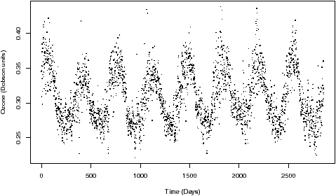
Design an application of multi-layer perceptron to predict the ozone levels into the future and report your design choices specifying inputs and outputs for the problem and consequently the input and output nodes for the network.

Naive Bayes.

Consider the binary classification problem of spam email in which a binary label Y ∈ {0, 1} is to be predicted from a feature vector X = (X₁, X₂, …, X_n), where X_i=1 if the word i is present in the email and 0 otherwise. Consider a naive Bayes model, in which the components X_i are assumed mutually conditionally independent given the class label Y.

[a] Draw a directed graphical model corresponding to the naive Bayes model.
Find a mathematical expression for the posterior class probability p(Y = 1 | x), in terms of the prior class probability p(Y = 1) and the class-conditional densities p(x_i | y).
Make now explicit the hyperparameters of the Bernoulli distributions for Y and X_i. Call them, µ and θ_i, respectively. Assume a beta distribution for the prior of these hyperparameters and show how to learn the hyperparameters from a set of training data d=(y^j,x^→j)_j=1^m using a Bayesian approach. Compare this solution with the one developed in class via maximum likelihood.

Consider again a naive Bayes for spam classification. How things would change wrt the previous exercise if the feature vector for a an email j were now X^j = (X₁^j, X₂^j, …, X_nj^j), with n_j the number of words in the email and X_i^j ∈ {1,…,N} no longer binary but indicating a number that corresponds to the word that appears in the ith position.

Neural Networks Make a McCulloch-Pitts neuron or a multilayer network that can calculate the logic function double implication: ⇔.

A joint probability table for the binary variables A, B, and C is given below.

A / B b₁ b₂

a₁ (0.006, 0.054) (0.048, 0.432)

a₂ (0.014, 0.126) (0.032, 0.288)

Table 2: Joint probability distribution P (A, B, C)

Calculate P (B, C) and P (B).
Are A and C independent given B? (Remember to report the justification of your answer.)

A / B	b₁	b₂

a₁	(0.006, 0.054)	(0.048, 0.432)
a₂	(0.014, 0.126)	(0.032, 0.288)