x=A \ b and y=inv(A)*b) in the same
plot. Try log-transformations until the curves resemble a line. (Find
size of matrices that allow to see differences in the results,
alternatively make a loop in which the same operation is repeated
several times, then the time for performing the operation once is the
average time.)| R(r) = r +n × (n × r ) ( 1−cos(φ) ) +( n × r ) sin(φ), (1) |
- How many real numbers do you need to specify a rotation in 3D?
- The matlab program rotate.m produces
Fig. 1. Read the script and understand what it is
doing. Modify the program to produce similar figures with different
rotation axes.
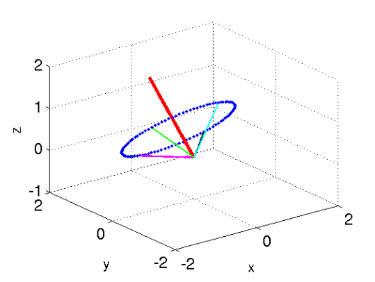
Figure 1: The figure is obtained using Eq. 1. The thick axis is the rotation axis. - Find the matrix of R in the standard basis.
-
Here we only introduce and use the definition: v is a
(right) eigenvector of the matrix L if and only if
it satisfies the equation
where λ is a scalar.L v = λ v, (2) Show that the rotation axis n is an eigenvector of the rotation operator. What ts the corresponding eigenvalue? Give a physical interpretation.
An important model in this field is the logistic equation or Verhulst equation
| y′=y−y2, y(0)=0.2 |
that expresses the rate of growth of the population y over time t (dy/dt=y′). The first term on the right hand side, y, determines a positive growth. If the model was just y′=y then the growth would be exponential and unlimited (you can verify this claim by deriving the solution of the equation). The second term, −y2, is a “braking term” that prevents the population from growing without bound. Finally, y(0) is the initial value, needed to solve the equation.
The logistic equation above is a nonlinear nonhomogeneous ordinary differential equation (ODE) (see Chapter 1 of [Kr] for an explanation of these terms). That specific equation can be reduced to a linear form and the solution written down as a formula (that is, in closed form). If you do not remember or do not know how to derive the closed form of that equation, you can read on page 30 of [Kr].
However, often a closed form is not known. Computational methods have then been developed for a numerical solution of the equation. More specifically, in MatLab there is a set of functions for carrying out this task in the case of ODEs. To gain an idea of the algorithms they implement you can read Section 21.1 of [Kr]. A distinction is done between stiff and nonstiff functions. The name is taken from one of the main applications of ODEs, which is in the study of oscillations. It is related to the value of the constants involved in the ODE. The term stiff recalls a mass-spring system with a stiff spring (large constant k). For stiff functions methods must be more accurate in order to avoid an increase in errors from the initial value.
- Search in the MatLab Help for “Ordinary Differential Equations”.
- Retrieve from the source given above the closed form solution of the equation.
- Compare in a plot the closed form solution with the solution
provided by some of the MatLab functions. In particular, try the
ode23andode23s. Which is giving the best solution? - Provide an interpretation of the curve observed from a physical point of view.