by Jarno Markku Olavi Rantaharju
Contents
Closed from solution
The equation y' = y - y^2 can be solved with the substitution v = 1/y. Then v' = 1/y^2 y' and substituting this to the equation gives v' = v - 1. This is solved by v=1 and the homogeneous equation v' -v = 0 is solved by v = C*exp(-t). The full set of solutions is then v = 1 + C*exp(-t)
Substituting this back to v=1/y equation then gives y = 1/(1+C*exp(-t))
The initial condition is y(0) = 0.2. Substituting this to the solution gives y(0) = 1/(1+C) = 0.2 Solving for C we get C = 4 And finally y = 1/(1+4*exp(-t))
To plot the closed form solution we need to find it at a set of points t First define a set of point t
t=[0:0.01:10];
and then find y at each t
y = 1./(1+4*exp(-t));
and plot
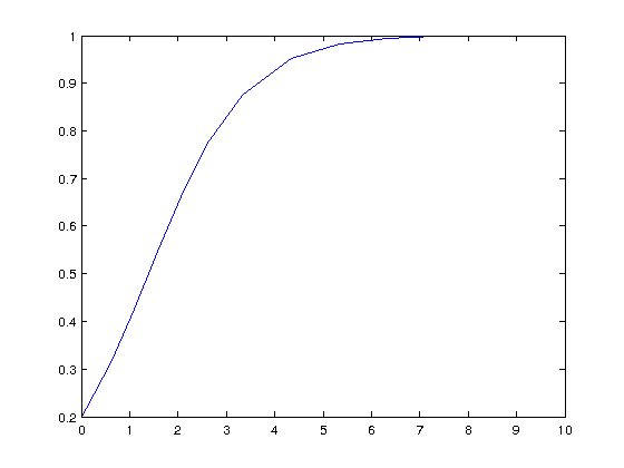
plot(t,y)

The function y(t) descripes the population of a species as a function of time. Initially the population grows exponentially, for a small while, but the braking term starts to slow the growth down between t=1 and t=2. We see the population reaching a balance where it no longer changes after t=7.
At the balanced state, y=1, the population no longer changes since y' = y - y^2 = 1-1 = 0.
Using ode23
Matlab can solve differential equations numerically with a few functions, for example ode23, ode23s and ode45. There is more information in the documentation (see doc ode23). The function needs an initial condition such as y(t0) = y0. In this case t0=0 and yo=0.2.
t0=0;
y0 = 0.2;
We also need the highest value of t we want the solution at, t1
t1=10;
We also need a function that returns y'. This needs to be in a separate file. I want to call the function Polulation_dy, so I need to make a file called Population_dy.m . The file contains the next three lines (without the % signs ):
%function [ dy ] = Population_dy( t, y )
%     dy = y - y.^2;
% end
Now we can call the function to solve the equation. It will return the solution as a set of points t2 and y2.
tspan=[t0,t1];
[t2,y2] = ode23(@Population_dy,tspan,y0);
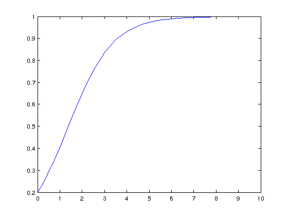
If we didn't specify the point t2 and y2, we the ode23 would produce a plot of the solution. We can plot it with
plot(t2,y2)
Using ode23s
The function ode23s is called in the same way. It uses a different algorithm to find the solution
[t3,y3] = ode23s(@Population_dy,tspan,y0);
Plot the points (t3,y3)
plot(t3,y3)
Using ode45
The function ode45 uses another algorithm.
[t4,y4] = ode45(@Population_dy,tspan,y0);
Plot
plot(t4,y4)

This seem to be closest to the exact solution