DM204 – Scheduling, Timetabling, Routing
Assignment Sheet 1, Fall 2010 [pdf format]

Prepare for discussion in class at 10.00 of Wednesday, February 17 as many of these exercises as you can. Proceed in the presentation order.

Preface to exercises 1 to 6

In a combinatorial optimization problem (COP) we are typically given a finite set N={1,…,n} of objects, weights c_j for each j∈ N and a set F of feasible subsets of N. The task is finding a minimum weight feasible subset, that is,

Items 1 to 6 below are COPs that you have to formulate as a (Linear) Mixed Integer Program, a (Linear) Integer Program, or a Binary Integer Program.

Make a clear distinction between the data of the problem instance and the variables (unknowns used in the model). Then, (i) Define what appear to be the necessary variables; (ii) Use these variables to define a set of constraints so that the feasible points correspond to the feasible solutions of the problem; (iii) Use these variables to define the objective function. If difficulties arise define and additional or alternative set of variables and iterate. In COPS, we are often interested in choosing a subset S⊆ N. For this often it helps using the incidence vector of S, which is the n-dimensional 0–1 vector x^S such that x_j^S=1 if j ∈ S and x_j^S otherwise.

1. 0–1 Knapsack Problem There is a budget b available for investment in projects during the coming year and n projects are under consideration, where a_j is the outlay for project j, and c_j is its expected return. The goal is to choose a set of projects so that the budget is not exceeded and the expected return is maximized.
2. Set Covering Problem (SCP) Given a certain number of regions, the problem is to decide where to install a set of emergency service centers. For each possible center the cost of installing a service center, and which regions it can service are known. For instance if the centers are fire stations, a station can service those regions for which a fire engine is guaranteed to arrive on the scene of a fire within 8 minutes. The goal is to choose a minimum cost set of service centers so that each region is covered. More abstractly, Let M={1,…,m} be the set of regions, and N={1,…,n} the set of potential centers. Let S_j ⊆ M be the regions that can be serviced by a center at j∈ N, and c_j its installation cost. We obtain the problem: min_{T⊆ N} { ∑_{j∈ T} c_j : ∪_{j ∈ T} S_j = M}.
3. Traveling Salesman Problem (TSP). A salesman must visit each of n cities exactly once and then return to his starting point. The time taken to travel from city i to city j is c_ij. Find the order in which he should make his tour so as to finish as quickly as possible.
4. Uncapacited Facility Location (UFL) Given a set of potential depots N={1,…,n} and a set M={1,…,m} of clients, suppose there is a fixed cost f_j associated with the use of depot j and a transportation cost c_ij if all of client i’s order is delivered from depot j. The problem is to decide which depots to open and which depot serves each client so as to minimize the sum of the fixed and transportation costs.
5. Uncapacited Lot-Sizing (ULS)

   The problem is to decide on a production plan for an n-period horizon for a single product. The basic model can be viewed as having data:

   • f_t is the fixed cost of producing in period t.
   • p_t is the unit production cost in period t.
   • h_t is the unit storage cost in period t.
   • d_t is the demand in period t.
6. Job Shop Model Jm | | C_max in two ways: with discrete time variables and with continuous time variables. One of these models leads to disjunctive constraints. Show how they can be linearized.

   
   
   

7. Modelling disjunctions:
   • Extend the formulation saw in class for discrete alternatives to the union of two polyhedra P_k={x ∈ Rⁿ : A^k x ≤ b^k, 0 ≤ x ≤ u} for k=1,2, where M≥ max_kmax_i{a_i^kx−b_i^k : 0≤ x ≤ u}
   • Extend the formulation at the previous point to model that at of the constraints ∑_j=1ⁿ a_ij x_j ≤ b_i, i = 1,…,k at least h<k are satisfied.
8. Formulate the following as mixed integer programs:
   • (a) u=min{x₁,x₂}, assuming that 0≤ x_j ≤ C for j=1,2
   • (b) v=|x₁−x₂| with 0≤ x_j≤ C, for j=1,2
   • (c) the set X∖{x^*} where X={x ∈ Zⁿ : Ax≤ b } and x^* ∈ X.
   • (d) z=xy, where x,y ∈ B.

   ---

   

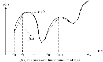
   Figure 1: Piecewise linear function f(x)

   ---

9. Piecewise linear functions. Many nonlinear programs can be piecewisely linearized and modelled as mixed integer programs. Consider a general nonlinear function g(x) of a single variable x. g(x) is continuous and x is within the interval [a₀,a_m]. Let f(x) be a piecewise linear function of g(x), where the interval [a₀,a_m] is partitioned into m small intervals via the break points [a₀,a₁,…,_m], where a₀ < a₁ < … < a_m as shown in Figure 1. Write the MIP program for the piecewise-linearized problem.