Mailing list: For enquiries, comments or bug reports, please register to the BaSTA Users mailing list
Cite as: Colchero, F., Jones, O.R and Rebke, M. (2012) BaSTA: an R package for Bayesian estimation of age-specific survival from incomplete mark-recapture/recovery data with covariates. Methods in Ecology and Evolution. 3: 466-470.
Latest news:
- BaSTA 1.9.5 available by clicking here (see installation instructions under Project Summary).
- BaSTA 1.9.4 is available on CRAN.
- Check additional functions in the EXTRA CODE section.
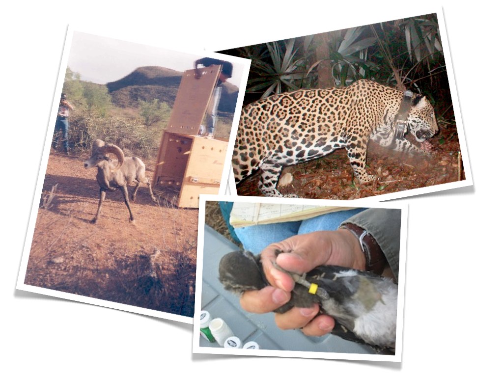
BaSTA, which stands for is "Survival Bayesian Trajectory Analysis", is an R package (R Development Core Team 2016) that allows users to draw inference on age-specific survival and mortality patterns from capture-recapture/recovery data when a large number of individuals (or all) have missing age information (Colchero, Jones and Rebke 2012). BaSTA is based on a model developed by Colchero and Clark (2012), which extends inference from parameter estimates to the estimation of unknown (i.e. latent) times of birth and death. The package also allows users to test the effect of categorical and continuous individual covariates on mortality and survival (for an example see Fig. 1).
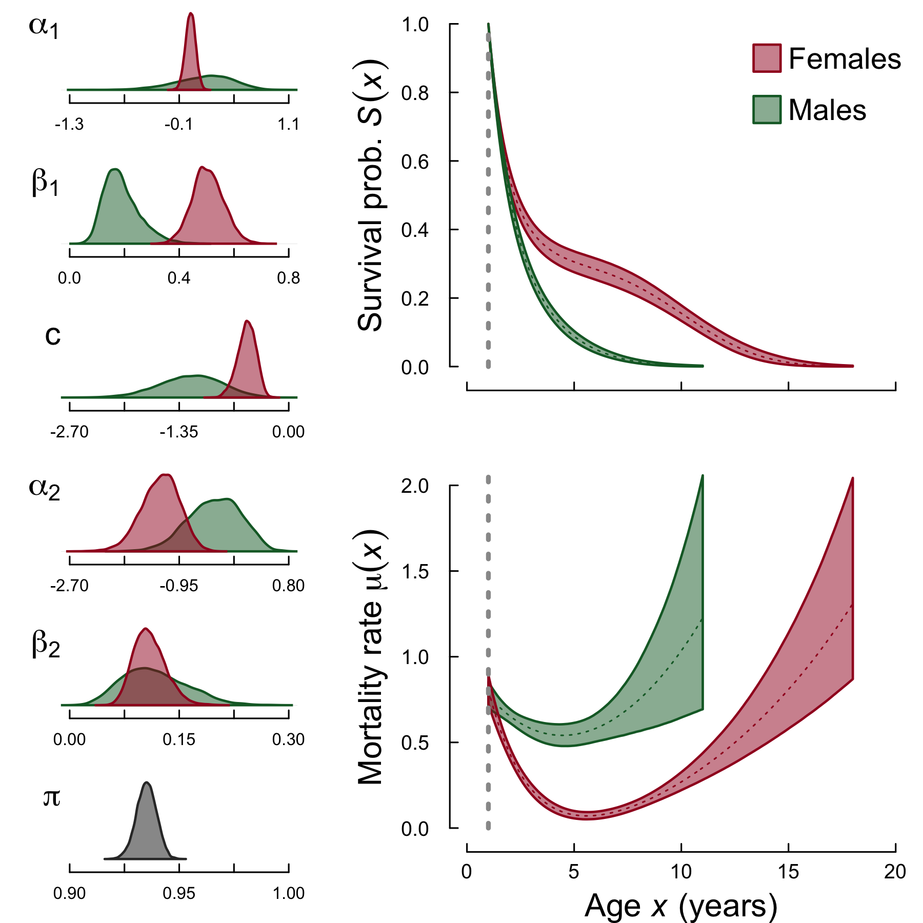
Fig. 1. BaSTA model output for sex differences in Soay sheep mortality using a Siler survival model (Colchero & Clark 2012). The left panel shows posterior distributions for the survival and recapture parameters while the right panel shows the resulting survival probabilities and the mortality rates for males and females.
Version 1.9.4 of the package is now availale on CRAN and can be installed by typing the following line of code into the R console:
install.packages("BaSTA")
Version 1.9.5 of the package is not yet availale on CRAN but can be downloaded by clicking here. Save the file in a folder of your choice, say ''C:/Documents/BaSTAtemp/'' for windows users, and then type on the R console:
install.packages("C:/Documents/BaSTAtemp/BaSTA_1.9.5.tar.gz", type = "source")
Alternatively the package can be install directly from our GitHub repository. To do so, first make sure to install the package "devtools" in R by typing:
install.packages("devtools")
Then, load the "devtools" library as:
library(devtools)
and install BaSTA as:
install_github("fercol/BaSTA/pkg")
This will always allow you to install the latest version of BaSTA.
We have set up a BaSTA Users mailing list so users can ask questions or provide comments, suggestions or criticism that can help us improve the package. Users can register by clicking here. Also, you can see below a video hosted by the journal Methods in Ecology and Evolution where we explain the rational behind the package and some general applications.
BaSTA video hosted by the journal Methods in Ecology and Evolution.
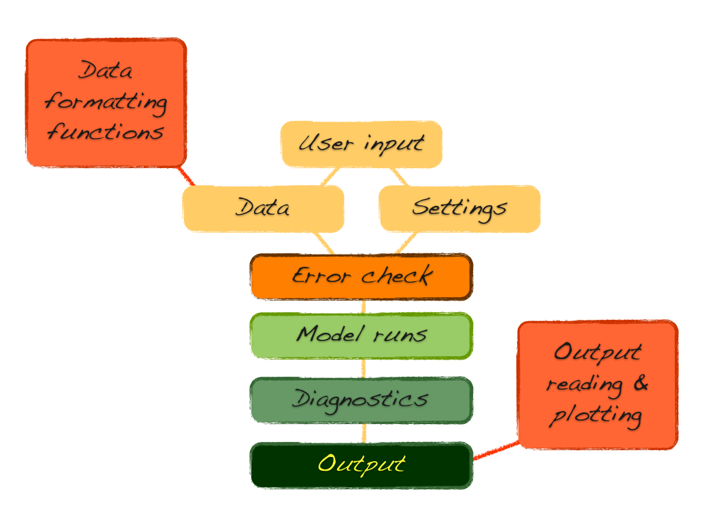
The core of the model is a Monte Carlo Markov Chain (MCMC) algorithm that combines Metropolis sampling for survival parameters and latent states (i.e. unknown times of birth and death) and direct sampling for recapture probabilities (Clark 2007, Colchero and Clark 2012). The main function performs several diagnostics on the user's inputs such as checking that the data is consistent with the model's requirements and verifies that the number of iterations, the burnin sequence and the thinning gap are consistent (Fig. 2).
Fig. 2. BaSTA general package chart.
After running these diagnostics, BaSTA uses a dynamic procedure to find adequate jump standard deviations for mortality parameters. This procedure runs before the core of the analysis is performed, keeping the user from having to find these jump sd's by trial and error. After apropriate jumps are found, multiple MCMC simulations can be ran either in parallel or in series. In case convergence is not acheived or some or all simulations failed, neither convergence nor model selection diagnostics are calculated.
The current version includes:
Functions for data formatting.
Data checking and correction of common data errors.
Estimates of age-specific survival parameters.
Estimates of yearly recapture probabilities.
Estimates of latent (i.e. unknown) times of birth and death.
Allows testing four different mortality functions (Exponential, Gompertz, Weibull and logistic) and to extend the model to Makeham or bathtub shapes (Gompertz 1925, Siler 1979, Cox and Oakes 1984, Pletcher 1999).
Evaluates the effects of time-independent categorical and continuous covariates on survival.
Runs multiple simulations either in parallel (using package snowfall; Knaus 2010) or in series.
Calculates basic diagnostics on MCMC performance such as parameter update rates and serial autocorrelation.
Uses multiple simulations to estimate convergence (i.e. potential scale reduction factor; Gelman et al. 2004).
Calculates basic measures for model fit (DIC; Spiegelhalter et al. 2002).
Finds jump standard deviations automatically through adaptive independent Metropolis (Roberts and Rosenthal 2009).
Future versions will include:
Time-dependent covariates.
Cohort effects on mortality
Covariates on recapture and recovery probabilities.
Extend the package for analyses on other types of data (e.g. census).
BaSTA is considerably easy to apply. The BaSTA vignette, which includes a step by step tutorial, can be accessed here. This vignette provides information on how to setup the dataset in an appropriate format for BaSTA and steps to run a range of analyses.
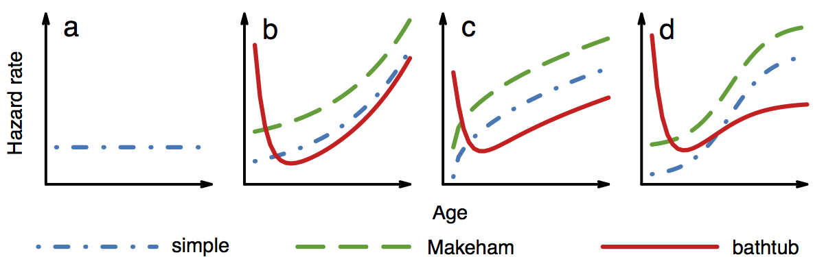
Here we provide a very general overview on the different analyses that can be performed with BaSTA and the types of outputs that the user should expect to find. As we mentioned above, BaSTA allows users to test a range of models and functional forms for the mortality function (Fig. 3).
Fig. 3. Functional forms that can be tested with BaSTA. The general types include: a) Exponential (the name is based on the survival probability); b) Gompertz; c) Weibull; and d) logistic. Additional shapes include Makeham (green dashed lines) and bathtub (red continous lines)
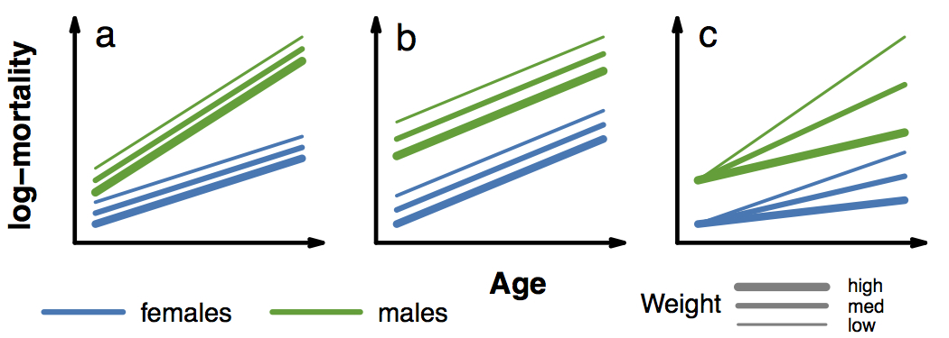
In addition, it is possible to test the effect of categorical and continuous covariates. In Fig. 4 we show examples on which effects can be tested with a combination of a categorical and a continuous covariates.
Fig. 4. Covariate effects that can be tested with BaSTA. Given two sets of covariates, one categorical (e.g. females vs males) and one continuous (e.g. weight) the effects that can be tested include: a) fused (i.e. categorical covariates affecting mortality parameters and continous covariates as proportional hazards); b) proportional hazards (both types of covariates as proportional hazards); and c) all in mortality (both covariates affecting mortality parameters; currently only implemented with Gompertz models)
After setting up the dataset, which we will call myDataset, and defining the years of start and end of the study, say, 1995 and 2005 respectively, a basic BaSTA analysis with a Gompertz mortality model (default) can be performed by typing into the R gui the following command:
In this case, BaSTA runs a single simulation for 11,000 iterations with a burn-in of 1001 steps. As we mentioned above, convergence can only be estimated by running more than one simulation. When running multiple simulations, we strongly recomend to use the routine that updates jump sd's. This will make the analysis sligthly longer, but will greatly increase the chances of getting convergence from the first try. To run 4 simulations of the same model as shown above with the jumps update routine on, the user only needs to type:
Argument parallel makes use of package snowfall (Knaus 2010), which allows BaSTA to run all 4 simulations in parallel, reducing computing time by a quarter of the time it would take to run each simulation one after the other.
Additional arguments such as model or shape can be used to test different functional forms for the mortality functions (Fig. 3). For instance, to run a logistic model with bathtub shape for 4 simulations in parallel, the code is:
If covariates are included in the dataset, the default is to run them as "fused" (see Fig. 4). To test different covariate effects, the user only needs to change argument covarsStruct. For example, to test the same model as above under a proportional hazards covariate structure the code should be modified as folows:
We recomend users to test different models, shapes and covariate structures and use the measures of model fit (i.e. DIC) for model comparison. In case the model does not converge, make sure that there are not too many missing records for younger individuals. This is commonly an issue with studies on birds, for which many juvenile individuals do not return to the breeding grounds when they reach maturity. To fix this without loosing information, BaSTA provides argument minAge that can be used to specify this minimum age. For example, the code for the model above with a minimum age of 1 is:
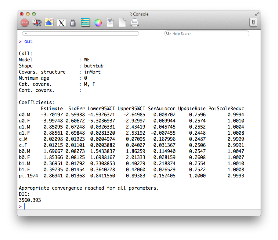
To visualize the result, the user only needs to type either out or, for additional information, function summary(out), which prints to the screen the relevant information such as the call of the model, the coefficients with standard errors and lower and upper bounds, if the model converged and if so, the value of model fit (DIC, which can be used for model selection; Fig. 5).
Fig. 5. BaSTA output printed by typing out into the R console. Additional information can be obtained by typing summary(out).
To visually assess convergence, the resulting traces for the parameters can be plotted by typing on the R console plot(out) (Fig. 6), which, as an example, produces the following figure for a Weibull model with bathtub shape and two covariates (males-M; females-F):
Fig. 6. Example of an output from a Weibull model with bathtub shape on a kestrel (Falco tinnunculus) dataset (Jones et al. 2008). The plot shows the traces for the mortality parameters for males (M) and females (F). The plot was produced with the R built-in function plot().
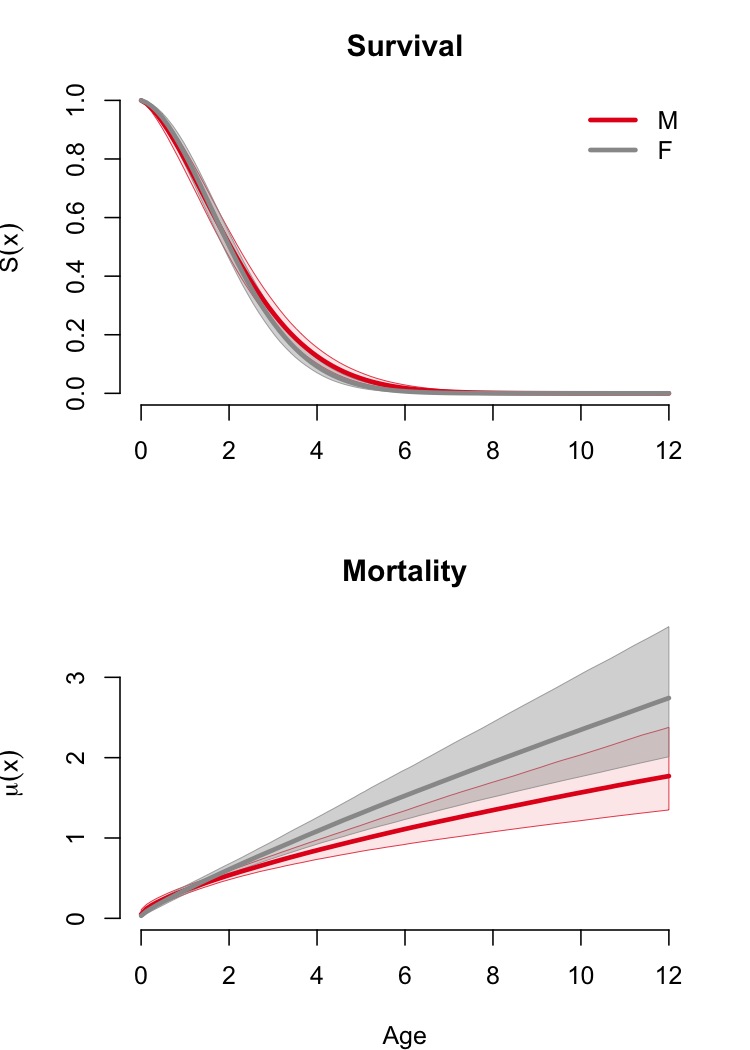
Also, the resulting mortality and survival probability trajectories (Fig. 7) can be plotted by typing plot(out, plot.trace = FALSE), producing the following plot for the same example:
Fig. 7. Survival probability and mortality trajectories for male (M) and female (F) kestrels (Falco tinnunculus).
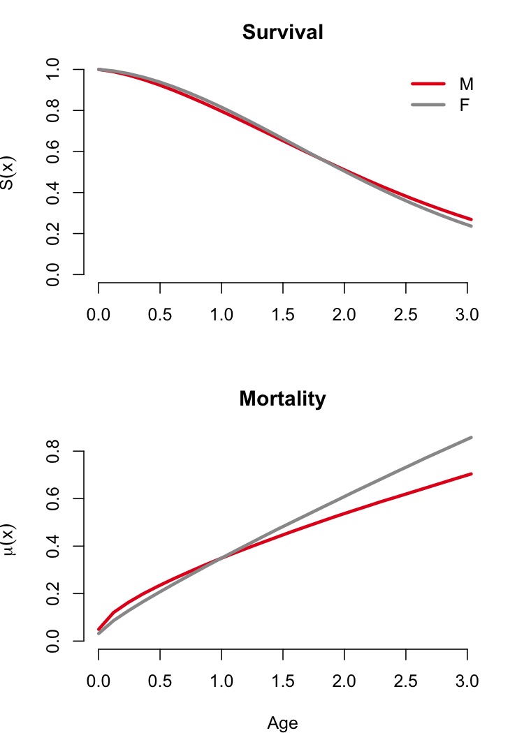
In case the survival and mortality plots become too crowded, which can happen if several categorical covariates are evaluated, function plot() can be modified using arguments xlim, which reduces the range of ages over which the plots are produced, and argument noCI, which eliminates credible intervals and only plots the mean expected trajectories (Fig. 8):
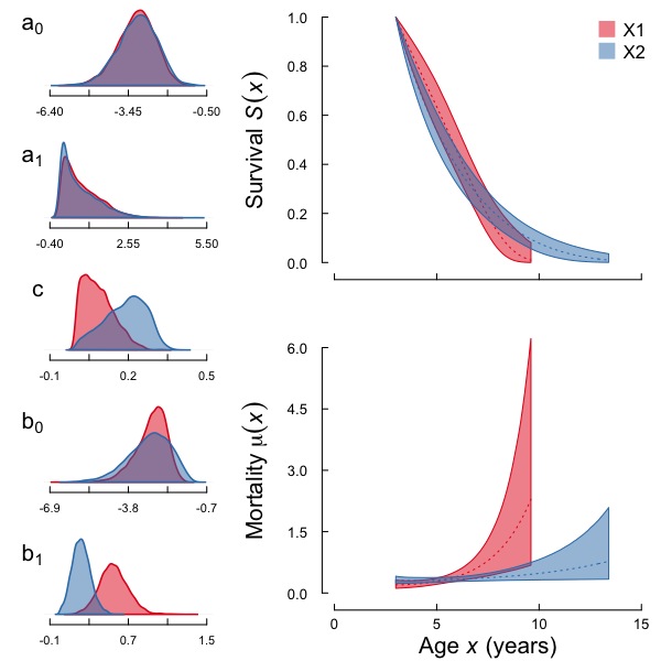
To create plots such as Fig. 9 that include the posterior density plots for the different parameters as well as the resulting survival and mortality profiles, you can modify function plot() as:
plot(out, fancy = TRUE)
which should produce a plot similar to Fig. 9 below.
Fig. 9. Density plots for a bathtub-logistic model and survival and mortality profiles for adult rooks (Corvus frugilegus) in locations X1 and X2 plotted using function plotFancyBaSTA() (Jones and Colchero in prep.).
Note that this function is compatible with outputs from BaSTA version 1.5 and higher. Also, it is meant to plot outputs from models that used values of all.in.mort and fused for the shape argument.
We have put together a set of functions that allow BaSTA users to run and compare several (or all) of the models featured in the package. The main function, called multibasta() uses the basic arguments as function basta() but also allows users to specify which models and shapes they wish to compare. To run all the models in BaSTA on a given dataset, say myData for a study starting in 2000 and finishing in 2010, only type the default commands into the R console:
If you wish to compare only a subset of the models, for example EX (exponential), GO (Gompertz) and WE (Weibull) models with simple shapes, you can type into the R console the folowing command:
To modify the basic BaSTA parameters, such as the number of iterations, the number of runs, etc., just use the same arguments you would use in function basta(). For instance, if you want to run 4 parallel sets of iterations for each model, just modify the code as follows:
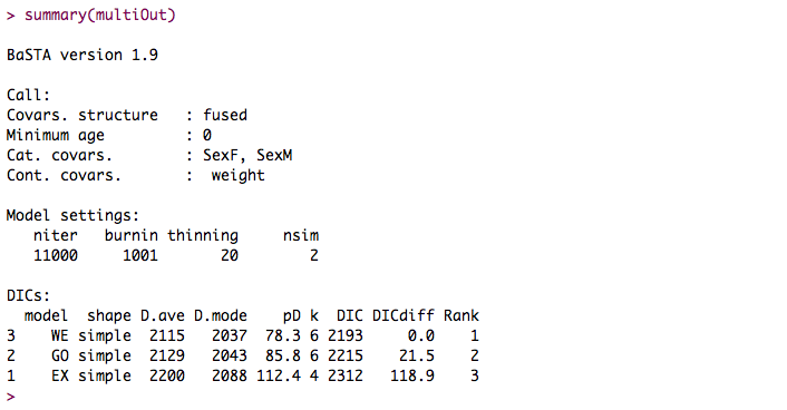
The same applies for any other argument. After function multibasta() finishes, you can visualise the basic results either by typing the name of the output in the R console, in this case multiOut, or by using the R function summary(multiOut). For example, the summary for a dataset with sex and weight as covariates and the models we specified above prints the following output to the console:
Fig. 10. Summary of output from function MultiBaSTA().
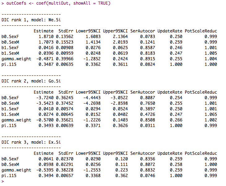
Also, it is possible to print and save the coefficients of any of the functions with the built-in function coef(). Thus, to print only the coefficients from the model with lowest DIC, only type coef(multiOut) to the console. In case you wish to print several of the model's coefficients use argument showAll as:
Fig. 11. Output from function coef() on a multibasta object.
Argument showAll can be modified to show only specific models, for instance, if you whish to print only the two models with lowest DIC, just type coef(multiOut, showAll = c(1, 2)). To view models not in consecutive order, only specify their ranking as show in the DIC table aftet typing multiOut in the R console.
Fixed bug in function CensusToCaptHist() where the IDs of individuals were incorrectly returned as the rows of the output data frame rather than those from the column called ID.
Fixed a bug in function mulitbasta() when arguments models and shapes were not specified.
BaSTA 1.9.4 In CRAN:
Fixed a bug that produced the following ''Error in FUN(newX[, i], ...) : invalid 'type' (character) of argument.'' when using covariates.
BaSTA 1.9.3(01/03/2014):
Fixed a bug in version 1.9.2 that in some cases assigned proposed ages at death to the wrong individuals.
BaSTA 1.9.2 (do not use this version) (25/01/2014):
Minor bug fixes.
BaSTA 1.9 (10/08/2013):
Fixed a bug when calculating the mean age at death that made mortality at the initial ages equal to 0 for some life tables.
Minor bug fixes.
BaSTA 1.8 (15/01/2013):
Fixed bug that lumped deaths at the minAge for individuals not seen after birth.
Changed the range of ages plotted in the surival and mortality plots to show the curves for ages such that S(x) > 0.01, this is, until only 1% of the cohort is still alive.
BaSTA 1.7 (28/12/2012):
Fixed bug that over-estimated ages at death and underestimated recapture probabilities with proportional hazards models.
BaSTA 1.6 (19/11/2012):
Fixed a bug that prevented to calculate quantiles for predicted mortality and survival when only continuous covariates were included.
Fixed a series of bugs when evaluating only continuous covariates inMort.
Fixed a bug that prevented to plot all the traces from proportional hazard parameters in the same plotting window.
Minor bug fixes.
BaSTA 1.5 (20/10/2012):
Great improvement on the updateJumps algorithm and the estimation of mortality parameters. This upgrade greatly reduces the number of iterations needed for convergence and the time required to run the analysis.
Fixed an issue when assigning times of birth and death that prevented the model to estimate deaths between ages 0 and 1.
Improved the plot() function to allow zooming to different ranges of ages when plotting survival and mortality and to plot these trajectories with or without credible intervals.
Minor bug fixes.
BaSTA 1.4 (25/09/2012):
Update jump routine for multiple simulations runs before the main analysis, this improves convergence and consistency between multiple simulations.
Improved convergence by fixing several bugs in the MCMC routine.
Fixed reporting of DIC values with function summary().
Function summary() ouputs the basic information, which can be stored instead of the main output. This reduces storage problems due to the size of the output.
Clark, J.S. (2007) Models for ecological data. Princeton University Press, Princeton, New Jersey, USA.
Colchero, F. and J.S. Clark (2012) Bayesian inference on age-specific survival for censored and truncated data.Journal of Animal Ecology, 81, 139-149 (publication).
Colchero, F., O.R. Jones and M. Rebke (2012) BaSTA: an R package for Bayesian estimation of age-specific survival from incomplete mark-recapture/recovery data with covariates.Methods in Ecology and Evolution. 3: 466-470 (publication).
Cox, D. R., and Oakes D. (1984) Analysis of Survival Data. Chapman and Hall, London.
Gelman, A., Carlin, J.B., Stern, H.S. & Rubin, D.B. (2004). Bayesian data analysis. 2nd edn. Boca Raton: Chapman & Hall/CRC.
Gimenez, O., Bonner, S., King, R., Parker, R.A., Brooks, S.P., Jamieson, L.E., Grosbois, V., Morgan, B.J.T., Thomas, L. (2009) WinBUGS for population ecologists: Bayesian modeling using Markov Chain Monte Carlo methods. In Modeling Demographic Processes in Marked Populations. Ecological and Environmental Statistics Series, vol 3 (eds D.L. Thomson, E.G. Cooch & M.J. Conroy), pp. 883-915. Springer, Berlin, Germany.
Gompertz, B. (1825) On the nature of the function expressive of the law of human mortality, and on a new mode of determining the value of life contingencies. Philosophical Transactions of the Royal Society of London, 115, 513-583.
Jones, O.R., Coulson, T., Clutton-Brock T. & Godfray, H.C.J. (2008) A web resource for the UK's long-term individual-based time-series (LITS) data. Journal of Animal Ecology 77: 612-615
King, R. and Brooks, S.P. (2002) Bayesian model discrimination for multiple strata capture-recapture data. Biometrika, 89, 785-806.
Barker, R.J. and Link, W.A (2010) Posterior model probabilities computed from model-specific Gibbs output. arXiv preprint arXiv:1012.0073.
Pletcher, S. (1999) Model fitting and hypothesis testing for age-specific mortality data. Journal of Evolutionary Biology, 12, 430-439.
R Development Core Team (2016). R: A language and environment for statistical computing. R Foundation for Statistical Computing, Vienna, Austria. ISBN 3-900051-07-0, URL http://CRAN.R-project.org/.
Roberts, G.O. and Rosenthal, J.S. (2009) Examples of adaptive MCMC. Journal of Computational and Graphical Statistics, 18, 349-367.
Siler, W. (1979) A competing-risk model for animal mortality. Ecology, 60, 750-757.
Spiegelhalter, D.J., Best, N.G., Carlin, B.P. & van der Linde, A. (2002) Bayesian measures of model complexity and fit. Journal of the Royal Statistical Society: Series B, 64, 583-639.