from numpy import *
from sympy import *
from fractions import Fraction as f
set_printoptions(precision=3,suppress=True)

def printm(a):
    """Prints the array as strings
    :a: numpy array
    :returns: prints the array
    """
    def p(x):
        return str(x)
    p = vectorize(p,otypes=[str])
    print(p(a))

def tableau(a,W=7):
    """Returns a string for verbatim printing
    :a: numpy array
    :returns: a string
    """
    if len(a.shape) != 2:
        raise ValueError('verbatim displays two dimensions')
    rv = []
    rv+=[r'|'+'+'.join('{:-^{width}}'.format('',width=W) for i in range(a.shape[1]))+"+"]
    rv+=[r'|'+'|'.join(map(lambda i: '{0:>{width}}'.format("x"+str(i+1)+" ",width=W), range(a.shape[1]-2)) )+"|"+
         '{0:>{width}}'.format("-z ",width=W)+"|"
         '{0:>{width}}'.format("b ",width=W)+"|"]
    rv+=[r'|'+'+'.join('{:-^{width}}'.format('',width=W) for i in range(a.shape[1]))+"+"]
    for i in range(a.shape[0]-1):
        rv += [r'| '+' | '.join(['{0:>{width}}'.format(str(a[i,j]),width=W-2) for j in range(a.shape[1])])+" |"]
    rv+=[r'|'+'+'.join('{:-^{width}}'.format('',width=W) for i in range(a.shape[1]))+"+"]
    i = a.shape[0]-1
    rv += [r'| '+' | '.join(['{0:>{width}}'.format(str(a[i,j]),width=W-2) for j in range(a.shape[1])])+" |"]
    rv+=[r'|'+'+'.join('{:-^{width}}'.format('',width=W) for i in range(a.shape[1]))+"+"]
    print('\n'.join(rv))
Exercise 1
Find all basic feasible solutions. Find a basis $B$ of size m, s.t. $x_B=A^{-1}_Bb\ge 0$, so $A_B$ must be non-singular.
Create all 3-combinations of 7 numbers. This is the set of all possible B's
Check if $A_B^{-1}$ exist.
$x_B=A^{-1}_Bb$ each $x_i\ge0$ for $i\in B$.
from scipy.linalg import *
from itertools import *
from numpy import *

A = array([[2,0,1,-4],[0,1,0,2],[0,0,1,0]])
I = identity(3)
A = concatenate([A,I],axis=1)
b = array([3,1,1])

for e in combinations(range(7),3):
    if(det(A[:,e]) != 0):
        x = dot(inv(A[:,e]),b)
        if(any(x<0)==False):
            print("_______________________")
            print()
            print("B =",e)
            print("x =",x)
Exercise 2
$\bullet$ We add the slack variables $x_4,x_5,x_6$ with $I=\{1,...,6\}$ and the equational standard form will be:
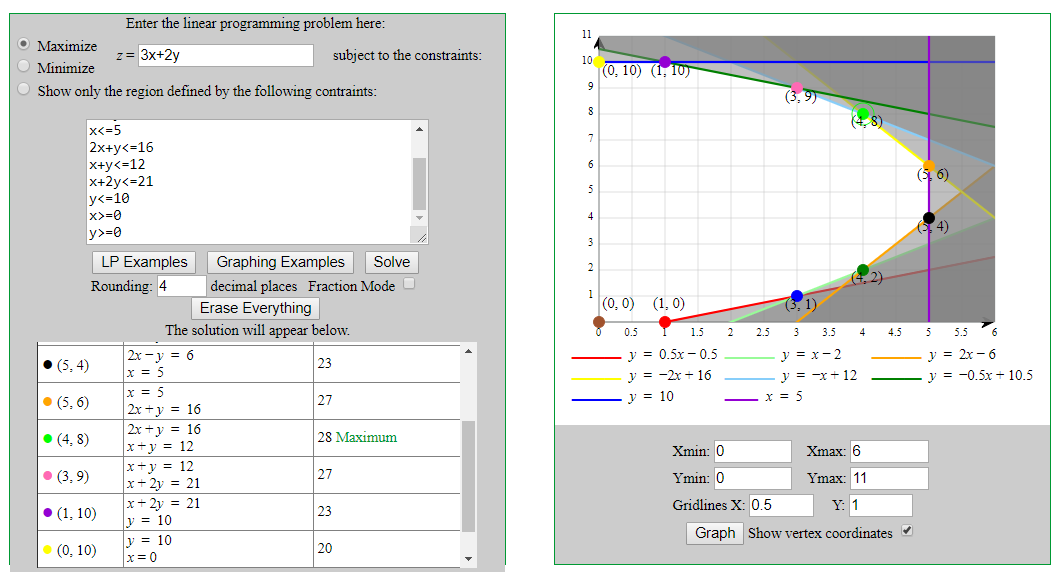
The LP model:
$\begin{aligned} \text{max} & \qquad 2x_1+4x_2-x_3 & \\ \text{s.t} & \qquad 2x_1-x_3+x_4 = 6 & \\ & \qquad 3x_2-x_3+x_5 = 9 & \\ & \qquad x_1+x_2+x_6 = 4 & \\ & \qquad x_i \ge 0 & \forall i \in \{1,...,6\} \\ \end{aligned}$
The first simplex tableau:
| _ | $x_1$ | $x_2$ | $x_3$ | $x_4$ | $x_5$ | $x_6$ | $-z$ | $b$ |
|---|---|---|---|---|---|---|---|---|
| $x_4$ | 2 | 0 | -1 | 1 | 0 | 0 | 0 | 6 |
| $x_5$ | 0 | 3 | -1 | 0 | 1 | 0 | 0 | 9 |
| $x_6$ | 1 | 1 | 0 | 0 | 0 | 1 | 0 | 4 |
| _ | 2 | 4 | -1 | 0 | 0 | 0 | 1 | 0 |
$\bullet$ $x_2$ has a reduced cost $>0$. Then the pivot column: 2. We find $r$ :
$r = argmin_i \left\{ \frac{b_i}{a_{is}}: \ a_{is}>0 \right\}$
print(9/3)
print(4/1)
Then $r=3$ which is $i=2$ and the we have pivot row: 2.
from numpy import *
A = array([[f(2,1),0,-1,1,0,0,0,6],[0,3,-1,0,1,0,0,9],[1,1,0,0,0,1,0,4],[2,4,-1,0,0,0,1,0]])
tableau(A)
A[1,:]=f(1,3)*A[1,:]
A[2,:]=A[2,:]-A[1,:]
A[3,:]=A[3,:]-4*A[1,:]
tableau(A)
$ \bullet$ This is the optimal solution since the reduced costs are non-positive.
print(6/2)
print(1/1)
Pivot: Column: 1, row: 3
A[0,:]=A[0,:]-2*A[2,:]
A[3,:]=A[3,:]-2*A[2,:]
tableau(A)
$x_1=1$
$x_2=3$
$x_3=0$
$x_4=4$
$x_5=0$
$x_6=0$
$z = 14$
Exercise 3
A=array([[2,f(3,1),1,1,0,0,0,5],[4,1,2,0,1,0,0,11],[3,4,2,0,0,1,0,8],[5,4,3,0,0,0,1,0]])
tableau(A)
Let $x_1$ enter.
$r = argmin_i \left\{ \frac{b_i}{a_{is}}: \ a_{is}>0 \right\}$
Find pivot.
print(5/2)
print(11/4)
print(8/3)
The pivot is column 1 row 1 with value: $r=2$ Let $x_4$ leave.
A[0,:] = f(1,2)*A[0,:]
A[1,:] = A[1,:]-4*A[0,:]
A[2,:] = A[2,:]-3*A[0,:]
A[3,:] = A[3,:]-5*A[0,:]
tableau(A)
Find new pivot. Let $x_3$ enter.
print(f(5,2)/f(1,2))
print(f(1,2)/f(1,2))
So the pivot column is 3 and pivot row is 3 with pivot value $1/2$. Let $x_6$ leave.
A[2,:]=2*A[2,:]
A[0,:]=A[0,:]-f(1,2)*A[2,:]
A[3,:]=A[3,:]-f(1,2)*A[2,:]
tableau(A)
$x_1 = 2$
$x_3 = 1$
$x_5 = 1$
$z = 13$
Exercise 4
Initial soluition of simplex is $x_1,x_2=0$, the clairvoyant rule say we should take the shortests path. If we take $x_2$ into basis we get a path of 4 arcs.
If we put $x_1$ into basis, we get a path of 6 arcs.
Exercise 5
Let $I=\{A,B,C,D,E,F\}$ be the set of activities. Let $x_i$ be the amount of weeks we want to shorten activity $i$. Let $y_i$ be the earliest activity $i\in I$ can start. Let $y_{end}\le 19$ denote the ending activity. The objective is to minimize the cost of shortening the duration of each activity. Let $d_i$ be the normal time that activity $i$ starts, then we add the constraints: $y_j\ge y_i+(d_i-x_i)$ for each arc $i\rightarrow j$ such that activity $j$ cannot start before all predecessors $i$ have finished.
The LP model:
$\begin{aligned} \text{min} & \qquad 6x_A+10x_B+8x_D+8x_E+3x_F & \\ \text{s.t} & \qquad y_C \ge y_A+(7-x_A) & \\ & \qquad y_C \ge y_B+(10-x_B) & \\ & \qquad y_D \ge y_A+(7-x_A) & \\ & \qquad y_D \ge y_B+(10-x_B) & \\ & \qquad y_E \ge y_C+5 & \\ & \qquad y_E \ge y_D+(3-x_D) & \\ & \qquad y_F \ge y_C+5 & \\ & \qquad y_F \ge y_D+(3-x_D) & \\ & \qquad y_{end} \ge y_E+(8-x_E) & \\ & \qquad y_{end} \ge y_F+(7-x_F) & \\ & \qquad y_{end} \le 19 & \\ & \qquad x_A \le 2 & \\ & \qquad x_B \le 5 & \\ & \qquad x_C \le 0 & \\ & \qquad x_D \le 2 & \\ & \qquad x_E \le 2 & \\ & \qquad x_F \le 3 & \\ & \qquad x_i \ge 0 & \forall i \in I \\ & \qquad y_i,y_{end} \ge 0 & \forall i \in I \\ \end{aligned}$
from pyscipopt import *
import numpy as np
m = Model("activity")
c = [6,10,0,8,8,3]
b = [2,5,0,2,2,3]
ir = range(6)
# ir = [A,B,C,D,E,F]
# ir = [0,1,2,3,4,5]
jr = range(7)
x = {}
y = {}
# Variables
for i in ir:
    x[i] = m.addVar(vtype = "C", name = "x(%s)" % i)
for j in jr:
    y[j] = m.addVar(vtype = "C", name = "x(%s)" % j)
# Objective
m.setObjective(quicksum(c[i]*x[i] for i in ir),"minimize")
# Constraints
# C
m.addCons(y[2] >= y[0]+(7-x[0]))
m.addCons(y[2] >= y[1]+(10-x[1]))

# D
m.addCons(y[3] >= y[0]+(7-x[0]))
m.addCons(y[3] >= y[1]+(10-x[1]))
# E
m.addCons(y[4] >= y[2]+5)
m.addCons(y[4] >= y[3]+(3-x[3]))
# F
m.addCons(y[5] >= y[2]+5)
m.addCons(y[5] >= y[3]+(3-x[3]))
# end
m.addCons(y[6] >= y[4]+(8-x[4]))
m.addCons(y[6] >= y[5]+(7-x[5]))
m.addCons(y[6] <= 19)
for i in ir:
    m.addCons(x[i]<=b[i])
    m.addCons(x[i]>=0)
for j in jr:
    m.addCons(y[j]>=0)


m.optimize()

print("obj: ", m.getObjVal())
print()
for j in jr:
    print("y[%s] = %s" % (j,m.getVal(y[j])))
print()
for i in ir:
    print("x[%s] = %s" % (i,m.getVal(x[i])))
Exercise 6
1.: 4. In nD, it takes n intersecting hyperplanes to get a point.
2.: Yes.
3.: When the planes are linearly independent.
4.: At least the amount variables, which is $n$.
5.: Not if the vertex is outside the feasible region.
6.: Yes. For example in 3D if we have a pyramid formed by 4 constraints.
7.: No.
$x_1+x_2$
$x_1+x_2\le 1$
8.: A cube in 3-dimensional we need $3n=3*2=6$ constraints which have $2^n=2^3=8$ vertices. For an $n-hypercube$ we need $2n$ constraints and $2^n$ vertices.
9.: The upper bound is ${m \choose n}=\frac{m!}{n!(m-n)!} $
10.: True, False, False.
11.: At most two can be different from zero, since we have two constraints.
Both constraints are active.
At most m
$n-m$, at most $m<n$ products
12.: Since $x_4=0$ is the slack variable of the second constraint it is active.
13.: 3 constraints would be active.
14.: True
15.: Then one basic variable is zero. Can draw 2D for:
$x_1+x_2\le 1, \ x_1\le 1, \ x_i \ge 0$
16.:
For 2 dimensions: they have 1 constraint in common.
For 3 dimensions: they have 2 constraints in common.
For n dimensions: they have $ n-1$ constraints in common.
Then we need $n-1$ common variables in basis.
(3*2)/(2*(3-2))
A=array([[f(1,1),1,1,0,0,1],[1,0,0,1,0,1],[1,1,0,0,1,0]])
tableau(A)
A[1,:]=A[1,:]-A[0,:]
A[2,:]=A[2,:]-A[0,:]
tableau(A)
$x_1=1$
$x_2=0$
$x_3=0$
$x_4=0$
Exercise 7
Thm 2.5: If the simplex fails to terminate, then it must cycle. Proof. A tableau is determined by which var. is in base and which are not. There are ${n+m \choose m}$ possibilites, hence finite. Then it will terminate if it does not cycle.
Then it cycles use Blend's rule to prevent this. Choose lowest index for entering variable and leaving.
Exercise 8
a.
A point is feasible if it is inside the feasible region.
A point is basic if there are the same amount of active constrainst as there are variables.
The points:
$i:$ is feasible.
$ii:$ is feasible.
$iii:$ is basic and feasible.
$iv:$ is basic.
b.
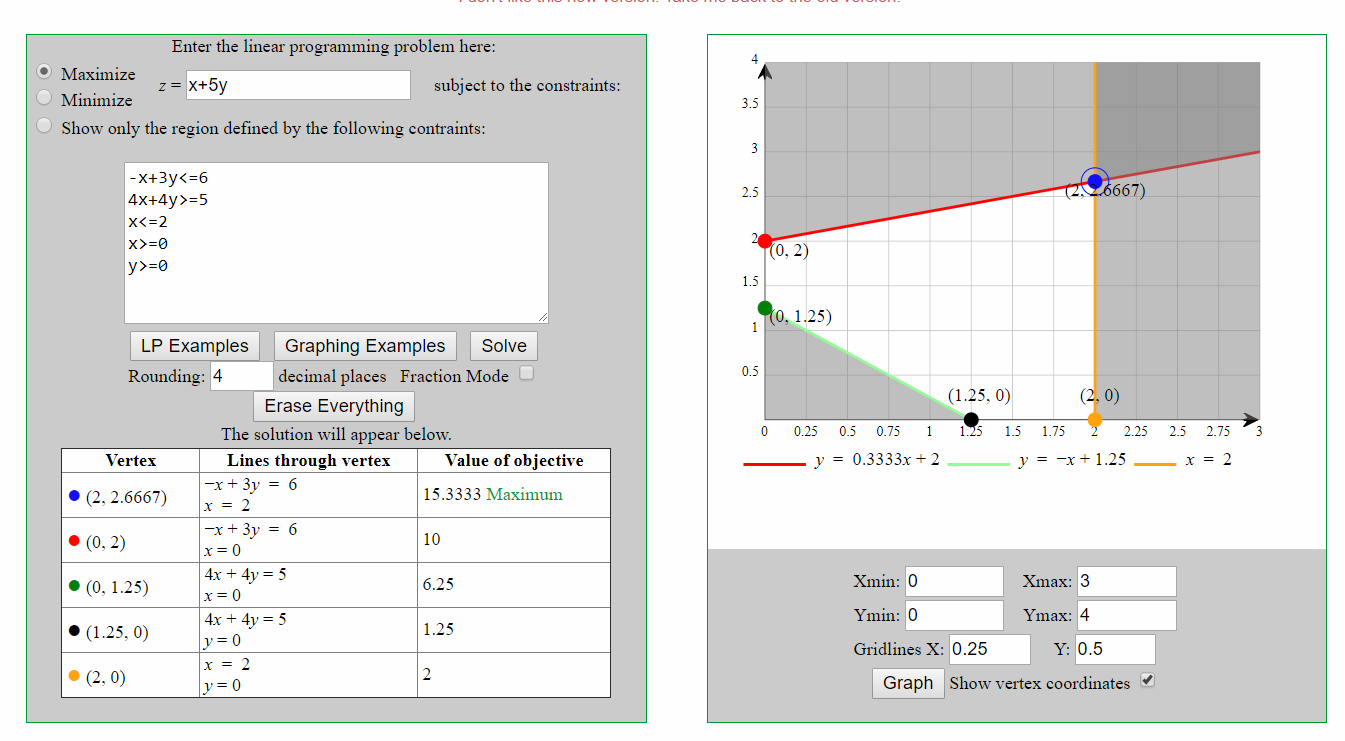
The LP model:
$\begin{aligned} \text{max} & \qquad z=x_1+5x_2 & \\ \text{s.t} & \qquad -x_1+3x_2 \le 6 & \\ & \qquad -4x_1-4x_2 \le -5 & \\ & \qquad x_1 \le 2 & \\ & \qquad x_i \ge 0 \\ \end{aligned}$
The basic solution is:
$x_1=0$
$x_2=0$
$x_3=6$
$x_4=-5$
$x_5=2$
$z=0+5*0=0$ it is not feasible and not optimal. Since the second constraint is violated.
A=array([[-1,3,1,0,0,0,6],[-4,-4,0,1,0,0,-5],[1,0,0,0,1,0,2],[1,5,0,0,0,1,0]])
tableau(A)
c.
$\bullet$ Largest coefficient consider $x_2, x_4$. With $x_2$ having largest coefficient we pick it. $x_1$ leaves.
A=array([[0,f(4,1),1,-f(1,4),0,0,f(29,4)],[1,1,0,-f(1,4),0,0,f(5,4)],[0,-1,0,f(1,4),1,0,f(3,4)],[0,4,0,f(1,4),0,1,-f(5,4)]])
tableau(A)
print(f(29,4)/4.)
print(f(5/4)/1.)
A[0,:]=A[0,:]-4*A[1,:]
A[2,:]=A[2,:]+A[1,:]
A[3,:]=A[3,:]-4*A[1,:]
tableau(A)
A[0,:]=f(4,3)*A[0,:]
A[1,:]=A[1,:]+f(1,4)*A[0,:]
A[3,:]=A[3,:]-f(5,4)*A[0,:]
tableau(A)
A[0,:]=A[0,:]+f(16,3)*A[2,:]
A[1,:]=A[1,:]+f(1,3)*A[2,:]
A[3,:]=A[3,:]-f(8,3)*A[2,:]
tableau(A)
It takes three steps.
$\bullet$ Largest increase: We are still considering $x_2,x_4$.
For $x_2$ the increase will be $\text{min}\left\{\frac{29/4}{4}, \frac{5/4}{1}\right \}*4 = 5$
For $x_4$ the increase will be $\text{min}\left \{\frac{3/4}{1/4} \right \}*1/4 = 3/4$.
This means that $x_2$ is entering and $x_1$ is leaving.
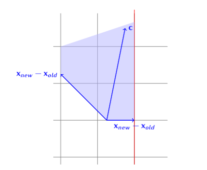
$\bullet$ Steepest edge
None of the rules are convenient, since they all take three steps. If we instead let $x_4$ enter and $x_5$ leave we reach the optimal solution in two steps.
A=array([[0,f(4,1),1,-f(1,4),0,0,f(29,4)],[1,1,0,-f(1,4),0,0,f(5,4)],[0,-1,0,f(1,4),1,0,f(3,4)],[0,4,0,f(1,4),0,1,-f(5,4)]])
tableau(A)
A[2,:]=4*A[2,:]
A[0,:]=A[0,:]+f(1,4)*A[2,:]
A[1,:]=A[1,:]+f(1,4)*A[2,:]
A[3,:]=A[3,:]-f(1,4)*A[2,:]
tableau(A)
A[0,:]=f(1,3)*A[0,:]
A[2,:]=A[2,:]+4*A[0,:]
A[3,:]=A[3,:]-5*A[0,:]
tableau(A)
Exercise 9
A = array([[0,f(1,1),1,0,0,5],[-1,1,0,1,0,1],[2,1,0,0,1,0]])
tableau(A)
The first is unbounded since the first column has positive reduced cost but no positive $a_{ij}$ term.
A = array([[f(5,1),10,1,0,0,60],[4,4,0,1,0,40],[1,1,0,0,1,0]])
tableau(A)
Let $x_2$ enter the basis.
print(60/10)
print(40/4)
Then $x_3$ leaves.
A[0,:]=f(1,10)*A[0,:]
A[1,:]=A[1,:]-4*A[0,:]
A[2,:]=A[2,:]-A[0,:]


tableau(A)
Let $x_1$ enter.
print(6/f(1,2))
print(16/2)
Let $x_4$ leave.
A[1,:]=f(1,2)*A[1,:]
A[0,:]=A[0,:]-f(1,2)*A[1,:]
A[2,:]=A[2,:]-f(1,2)*A[1,:]
tableau(A)
Optimal with $x_1=8, x_2=2, z=10$. We can see that $x_3$ have reduced cost 0. If we let $x_3$ enter and let $x_2$ leave.:
A[0,:]=5*A[0,:]
A[1,:]=A[1,:]+f(1,5)*A[0,:]
tableau(A)
Optimal with $x_1=10, x_3=10, z=10$
Convex combination:
$ x_1 = 8a+10(1-a)$
$ x_2 = 2a$
$ x_3 = 10(1-a)$
$ x_4 = 0$
Exercise 10
a. Since we have a negative b value, then $x_3=1, x_4=1$ is not feasible.
The LP model:
$\begin{aligned} \text{max} & \qquad z=4x_2 & \\ \text{s.t} & \qquad -2x_2+x_3 = 0 & \\ & \qquad 3x_1-4x_2+x_4 = -1 & \\ & \qquad x_i \ge 0 \\ \end{aligned}$
Make b positive.
$\begin{aligned} \text{max} & \qquad z=4x_2 & \\ \text{s.t} & \qquad -2x_2+x_3 = 0 & \\ & \qquad -3x_1+4x_2-x_4 = 1 & \\ & \qquad x_i \ge 0 \\ \end{aligned}$
from numpy import *
from fractions import Fraction as f
set_printoptions(precision=3,suppress=True)

def printm(a):
    """Prints the array as strings
    :a: numpy array
    :returns: prints the array
    """
    def p(x):
        return str(x)
    p = vectorize(p,otypes=[str])
    print(p(a))

def tableau1(a,W=7):
    """Returns a string for verbatim printing
    :a: numpy array
    :returns: a string
    """
    if len(a.shape) != 2:
        raise ValueError('verbatim displays two dimensions')
    rv = []
    rv+=[r'|'+'+'.join('{:-^{width}}'.format('',width=W) for i in range(a.shape[1]))+"+"]
    rv+=[r'|'+'|'.join(map(lambda i: '{0:>{width}}'.format("x"+str(i+1)+" ",width=W), range(a.shape[1]-3)) )+"|"+
         '{0:>{width}}'.format("-z ",width=W)+"|"+
         '{0:>{width}}'.format("-w ",width=W)+"|"
         '{0:>{width}}'.format("b ",width=W)+"|"]
    rv+=[r'|'+'+'.join('{:-^{width}}'.format('',width=W) for i in range(a.shape[1]))+"+"]
    for i in range(a.shape[0]-1):
        rv += [r'| '+' | '.join(['{0:>{width}}'.format(str(a[i,j]),width=W-2) for j in range(a.shape[1])])+" |"]
    rv+=[r'|'+'+'.join('{:-^{width}}'.format('',width=W) for i in range(a.shape[1]))+"+"]
    i = a.shape[0]-1
    rv += [r'| '+' | '.join(['{0:>{width}}'.format(str(a[i,j]),width=W-2) for j in range(a.shape[1])])+" |"]
    rv+=[r'|'+'+'.join('{:-^{width}}'.format('',width=W) for i in range(a.shape[1]))+"+"]
    print('\n'.join(rv))
b. Phase I of the auxiliary problem:
The LP model:
$\begin{aligned} \text{max} & \qquad w^*=-x_5 & \\ \text{s.t} & \qquad -2x_2+x_3 = 0 & \\ & \qquad -3x_1+4x_2-x_4+x_5 = 1 & \\ & \qquad x_i \ge 0 \\ \end{aligned}$
A = array([[0,-2,f(1,1),0,0,0,0,0],[-3,4,0,-1,1,0,0,1],[0,4,0,0,0,1,0,0],[0,0,0,0,-1,0,1,0]])
tableau1(A)
Turn it into canonical form
A[3,:]=A[3,:]+A[1,:]
tableau1(A)
The basis consists of $x_3, x_5$.
$x_3=0$
$x_5=1$
c.
i) Not feasible. Since the second constraint is violated: $-3*0+4*0=0\ge 1$
ii) $x_5=1, z=-1$ and there are reduced cost with positive value, so no.
iii) Yes, $x_3=0$ is a basic variable.
iv) It will terminate since the simplex terminates.
v) It will not be feasible if for the original problem the feasible region is empty.
vi) Let $x_2$ enter and $x_5$ leave.
A[1,:]=f(1,4)*A[1,:]
A[0,:]=A[0,:]+2*A[1,:]
A[2,:]=A[2,:]-4*A[1,:]
A[3,:]=A[3,:]-4*A[1,:]
tableau1(A)
Since $w^*=0$ we have a starting feasbile solution for the original problem.
$x_2=1/4$
$x_3=1/2$
We move to phase II by removing last row and columts $x_5,-z$.
A = A[:-1,[0,1,2,3,5,7]]
tableau(A)
For the first column have positive reduced cost but no positive $a_{ij}$ term, then the problem is unbounded.