from numpy import *
from numpy.linalg import inv
from fractions import Fraction as f
set_printoptions(precision=3,suppress=True)

def printm(a):
    """Prints the array as strings
    :a: numpy array
    :returns: prints the array
    """
    def p(x):
        return str(x)
    p = vectorize(p,otypes=[str])
    print(p(a))

def tableau(a,W=7):
    """Returns a string for verbatim printing
    :a: numpy array
    :returns: a string
    """
    if len(a.shape) != 2:
        raise ValueError('verbatim displays two dimensions')
    rv = []
    rv+=[r'|'+'+'.join('{:-^{width}}'.format('',width=W) for i in range(a.shape[1]))+"+"]
    rv+=[r'|'+'|'.join(map(lambda i: '{0:>{width}}'.format("x"+str(i+1)+" ",width=W), range(a.shape[1]-2)) )+"|"+
         '{0:>{width}}'.format("-z ",width=W)+"|"
         '{0:>{width}}'.format("b ",width=W)+"|"]
    rv+=[r'|'+'+'.join('{:-^{width}}'.format('',width=W) for i in range(a.shape[1]))+"+"]
    for i in range(a.shape[0]-1):
        rv += [r'| '+' | '.join(['{0:>{width}}'.format(str(a[i,j]),width=W-2) for j in range(a.shape[1])])+" |"]
    rv+=[r'|'+'+'.join('{:-^{width}}'.format('',width=W) for i in range(a.shape[1]))+"+"]
    i = a.shape[0]-1
    rv += [r'| '+' | '.join(['{0:>{width}}'.format(str(a[i,j]),width=W-2) for j in range(a.shape[1])])+" |"]
    rv+=[r'|'+'+'.join('{:-^{width}}'.format('',width=W) for i in range(a.shape[1]))+"+"]
    print('\n'.join(rv))


def tableau1(a,W=7):
    """Returns a string for verbatim printing
    :a: numpy array
    :returns: a string
    """
    if len(a.shape) != 2:
        raise ValueError('verbatim displays two dimensions')
    rv = []
    rv+=[r'|'+'+'.join('{:-^{width}}'.format('',width=W) for i in range(a.shape[1]))+"+"]
    rv+=[r'|'+'|'.join(map(lambda i: '{0:>{width}}'.format("x"+str(i+1)+" ",width=W), range(a.shape[1]-3)) )+"|"+
         '{0:>{width}}'.format("-z ",width=W)+"|"+
         '{0:>{width}}'.format("-w ",width=W)+"|"+
         '{0:>{width}}'.format("b ",width=W)+"|"]
    rv+=[r'|'+'+'.join('{:-^{width}}'.format('',width=W) for i in range(a.shape[1]))+"+"]
    for i in range(a.shape[0]-1):
        rv += [r'| '+' | '.join(['{0:>{width}}'.format(str(a[i,j]),width=W-2) for j in range(a.shape[1])])+" |"]
    rv+=[r'|'+'+'.join('{:-^{width}}'.format('',width=W) for i in range(a.shape[1]))+"+"]
    i = a.shape[0]-1
    rv += [r'| '+' | '.join(['{0:>{width}}'.format(str(a[i,j]),width=W-2) for j in range(a.shape[1])])+" |"]
    rv+=[r'|'+'+'.join('{:-^{width}}'.format('',width=W) for i in range(a.shape[1]))+"+"]
    print('\n'.join(rv))

def tableau2(a,W=7):
    """Returns a string for verbatim printing
    :a: numpy array
    :returns: a string
    """
    if len(a.shape) != 2:
        raise ValueError('verbatim displays two dimensions')
    rv = []
    rv+=[r'|'+'+'.join('{:-^{width}}'.format('',width=W) for i in range(a.shape[1]))+"+"]
    rv+=[r'|'+'|'.join(map(lambda i: '{0:>{width}}'.format("y"+str(i+1)+" ",width=W), range(a.shape[1]-2)) )+"|"+
         '{0:>{width}}'.format("-z ",width=W)+"|"
         '{0:>{width}}'.format("b ",width=W)+"|"]
    rv+=[r'|'+'+'.join('{:-^{width}}'.format('',width=W) for i in range(a.shape[1]))+"+"]
    for i in range(a.shape[0]-1):
        rv += [r'| '+' | '.join(['{0:>{width}}'.format(str(a[i,j]),width=W-2) for j in range(a.shape[1])])+" |"]
    rv+=[r'|'+'+'.join('{:-^{width}}'.format('',width=W) for i in range(a.shape[1]))+"+"]
    i = a.shape[0]-1
    rv += [r'| '+' | '.join(['{0:>{width}}'.format(str(a[i,j]),width=W-2) for j in range(a.shape[1])])+" |"]
    rv+=[r'|'+'+'.join('{:-^{width}}'.format('',width=W) for i in range(a.shape[1]))+"+"]
    print('\n'.join(rv))

def tableau3(a,W=7):
    """Returns a string for verbatim printing
    :a: numpy array
    :returns: a string
    """
    if len(a.shape) != 2:
        raise ValueError('verbatim displays two dimensions')
    rv = []
    rv+=[r'|'+'+'.join('{:-^{width}}'.format('',width=W) for i in range(a.shape[1]))+"+"]
    rv+=[r'|'+'|'.join(map(lambda i: '{0:>{width}}'.format("x"+str(i+1)+" ",width=W), range(a.shape[1]-3)) )+"|"+
         '{0:>{width}}'.format("-z ",width=W)+"|"+
         '{0:>{width}}'.format("-e ",width=W)+"|"+
         '{0:>{width}}'.format("b ",width=W)+"|"]
    rv+=[r'|'+'+'.join('{:-^{width}}'.format('',width=W) for i in range(a.shape[1]))+"+"]
    for i in range(a.shape[0]-1):
        rv += [r'| '+' | '.join(['{0:>{width}}'.format(str(a[i,j]),width=W-2) for j in range(a.shape[1])])+" |"]
    rv+=[r'|'+'+'.join('{:-^{width}}'.format('',width=W) for i in range(a.shape[1]))+"+"]
    i = a.shape[0]-1
    rv += [r'| '+' | '.join(['{0:>{width}}'.format(str(a[i,j]),width=W-2) for j in range(a.shape[1])])+" |"]
    rv+=[r'|'+'+'.join('{:-^{width}}'.format('',width=W) for i in range(a.shape[1]))+"+"]
    print('\n'.join(rv))
Exercise 1
We have the following problem:
The LP:
$\begin{aligned} \text{max} & \qquad z=x_1-x_2 & \\ \text{s.t} & \qquad x_1+x_2 \le 2 & \\ & \qquad 2x_1+2x_2 \ge 2 & \\ & \qquad x_1,x_2 \ge 0 & \end{aligned}$
In equational standard form:
$\begin{aligned} \text{max} & \qquad z=x_1-x_2 & \\ \text{s.t} & \qquad x_1+x_2+x_3 = 2 & \\ & \qquad 2x_1+2x_2-x_4 = 2 & \\ & \qquad x_1,x_2,x_3,x_4 \ge 0 & \end{aligned}$
This does not have a feasible starting solution.
Auxiliary approach: with Phase I:
Let $x_5\ge0$ be the auxiliary variable, then we have:
$\begin{aligned} \text{max} & \qquad w=-x_5 & \\ \text{s.t} & \qquad x_1+x_2+x_3 = 2 & \\ & \qquad 2x_1+2x_2-x_4+x_5 = 2 & \\ & \qquad x_1,x_2,x_3,x_4,x_5 \ge 0 & \end{aligned}$
And the tableau looks as follows:
A = array([[f(1,1),1,1,0,0,0,0,2],[2,2,0,-1,1,0,0,2],[1,-1,0,0,0,1,0,0],[0,0,0,0,-1,0,1,0]])
tableau1(A)
The tableau is not in canonical form, so add row 2 to row 4:
A[3,:] = A[3,:]+A[1,:]
tableau1(A)
Let $x_1$ enter the basis. We test which variable leaves (row 3 is not considered since it is an objective):
print("row 1:",2/1)
print("row 2:",2/2)
We take the minimum, so the pivot is column 1 row 2. So $x_5$ leaves:
A[1,:]=f(1,2)*A[1,:]
A[0,:]=A[0,:]-A[1,:]
A[2,:]=A[2,:]-A[1,:]
A[3,:]=A[3,:]-2*A[1,:]
tableau1(A)
The solution is optimal with $w=0$, so we remove the last row and the two columns: $x_5,-w$ and move to Phase II:
A = A[:-1,[0,1,2,3,5,7]]
tableau(A)
We make $x_4$ leave and let $x_3$ enter, the pivot is column 4 and row 1:
A[0,:]=2*A[0,:]
A[1,:]=A[1,:]+f(1,2)*A[0,:]
A[2,:]=A[2,:]-f(1,2)*A[0,:]
tableau(A)
The solution is optimal with $(x_1,x_2,x_3,x_4) = (2,0,0,2)$ with $z^* = 2$
The dual simplex:
The primal:
$\begin{aligned} \text{max} & \qquad z=x_1-x_2 & \\ \text{s.t} & \qquad x_1+x_2 \le 2 & \\ & \qquad 2x_1+2x_2 \ge 2 & \\ & \qquad x_1,x_2 \ge 0 & \end{aligned}$
Rewrite constraint:
$\begin{aligned} \text{max} & \qquad z=x_1-x_2 & \\ \text{s.t} & \qquad x_1+x_2 \le 2 & \\ & \qquad -2x_1-2x_2 \le -2 & \\ & \qquad x_1,x_2 \ge 0 & \end{aligned}$
The dual:
$\begin{aligned} \text{min} & \qquad 2y_1-2y_2 & \\ \text{s.t} & \qquad y_1-2y_2 \ge 1 & \\ & \qquad y_1-2y_2 \ge -1 & \\ & \qquad y_1,y_2 \ge 0 & \end{aligned}$
Rewrite to standard form:
$\begin{aligned} \text{max} & \qquad -2y_1+2y_2 & \\ \text{s.t} & \qquad -y_1+2y_2 \le -1 & \\ & \qquad -y_1+2y_2 \le 1 & \\ & \qquad y_1,y_2 \ge 0 & \end{aligned}$
Adding slack variables, we get the following tableau:
A = array([[-1,2,1,0,0,-1],[-1,2,0,1,0,1],[-2,2,0,0,1,0]])
tableau2(A)
The initial tableau is infeasible. We are allowed to change the objective function. So let $z_1 = -x_1-x_2$.
Then we would have the dual as:
$\begin{aligned} \text{max} & \qquad -2y_1+2y_2 & \\ \text{s.t} & \qquad -y_1+2y_2 \le 1 & \\ & \qquad -y_1+2y_2 \le 1 & \\ & \qquad y_1,y_2 \ge 0 & \end{aligned}$
Adding the slack variables $y_3,y_4$, we get the following tableau:
A = array([[-1,2,f(1,1),0,0,1],[-1,2,0,1,0,1],[-2,2,0,0,1,0]])
tableau2(A)
Now we have an initial solution and we can solve this. Let $y_2$ enter and $y_4$ leave:
A[1,:]=f(1,2)*A[1,:]
A[0,:]=A[0,:]-2*A[1,:]
A[2,:]=A[2,:]-2*A[1,:]
tableau2(A)
This tableau is optimal. Now we can write the tableau of the primal but also include the changed objective of the dual.
The primal problem with both objective functions:
A = array([[1,1,f(1,1),0,0,0,2],[-2,-2,0,1,0,0,-2],[1,-1,0,0,1,0,0],[-1,-1,0,0,0,1,0]])
tableau3(A)
The tableau for the dual simplex is optimal but not feasible. We look at the row with negative $b$ value and choose the column that minimizes the ratio test: $|c/a|$. It is the second row, which means that $x_4$ leaves. We choose between:
Column 1: $|-1/-2|=1/2$
Column 2: $|-1/-2|=1/2$.
Lets pick column 1. Let $x_1$ enter.
A[1,:]=-f(1,2)*A[1,:]
A[0,:]=A[0,:]-A[1,:]
A[2,:]=A[2,:]-A[1,:]
A[3,:]=A[3,:]+A[1,:]
tableau3(A)
The tableau is optimal for the dual simplex, so we have an initial feasible solution to the primal problem:
$x=(1,0,1,0)$.
Phase II: Now we can remove the second objective and then we have the following tableau for the primal simplex:
A = A[:-1,[0,1,2,3,4,6]]
tableau(A)
Let $x_4$ enter basis and $x_3$ exit:
A[0,:]=2*A[0,:]
A[1,:]=A[1,:]+f(1,2)*A[0,:]
A[2,:]=A[2,:]-f(1,2)*A[0,:]
tableau(A)
The tablue is optimal since all reduced cost are negative of the variables not in basis. The solution is:
$x = (2,0,0,2), \ \ z^* = 2 $
Which is the same as the previous found solution.
Exercise 2
a)
The initial tablue will look as follows:
from numpy import *

A = array([[3,2,1,2,1,0,0,0,225],[1,1,1,1,0,1,0,0,117],[4,3,3,4,0,0,1,0,420],[19,13,12,17,0,0,0,1,0]])
b = array([[225],[117],[420]])
tableau(A)
We have $B=\{x_1,x_3,x_4\}$, then $A_B$:
A_B = A[:-1,(0,2,3)]
print(A_B)
And $A_N$ will look as follows:
A_N = A[:-1,(1,4,5,6)]
print(A_N)
And $A_B^{-1}A_N$ will look as follows:
from numpy.linalg import inv
print(dot(inv(A_B),A_N))
Now want to find our final tableau. Our $b-values = A_B^{-1}b$:
x_B = dot(inv(A_B),b)
print(x_B)
We have $c_B, c_N$:
c = array([[19,13,12,17]])
c_B = array([[19],[12],[17]])
c_N = array([[13],[0],[0],[0]])
Our $z^* = -c_B^TA_B^{-1}b$:
dot(-c_B.T,dot(inv(A_B),b))
Our reduced cost for non basis varibles are found using $c_N^T-c_B^TA_B^{-1}A_N$:
c_N.T-dot(c_B.T,dot(inv(A_B),A_N))
Hence we have the final tableau:
AA = array([[1,1,0,0,1,2,-1,0,39],[0,1,1,0,0,4,-1,0,48],[0,-1,0,1,-1,-5,2,0,30],[0,-1,0,0,-2,-1,-3,1,-1827]])
tableau(AA)
All reduced costs are negative, which means that the solution is optimal.
b)
We look at the reduced cost in the final tableau for $x_2$ which is $-1$. If we increase the price for $x_2$ by more than $1$, then it would be worth producing.
c)
The shadow price is the negative of the coefficients of $x_5,x_6,x_7$ in the last row (also the dual values $y_1=2,y_2=1,y_3=3$), the marginal values:
For an extra hour of work: 2
For one extra amount of metal: 1
For one extra amount of wood: 3
d)
From the complementary slackness theorem we have:
$\begin{aligned} \left(b_i-\sum\limits_{j=1}^na_{ij}x_j^*\right)y_i^* = 0, \qquad i=1,...,m \end{aligned}$
Since $y_1,y_2,y_3>0$, then all constraints are binding.
e)
We are better off selling the raw materials that it takes to produce $x_2$, which is calculated as the dual values multiplied by the required material:
$\sum\limits_{i=1}^3y_ia_{i2}=2*2+1*1+3*3 = 14$ which is larger than the price $c_2=13$.
Solve the following variations:
1)
The net profit for $x_2$ increases from 13 to 15. We showed in b) that if the increase is larger than 1, $x_2$ will enter basis. So now we need to determine which variable should leave.
Step 1 and Step 2 is to determine the entering variable, which we have already done.
Step 3. We need to calculate $d = A_B^{-1}a$, for $d$ being the corresponding column of $x_2$ in $A$.
d = array([dot(inv(A_B),A_N[:,0])])
print("d =", d)
Step 4 Determine the largest $\theta$ s.t. $x_B = x_B'-d\theta \ge 0$.
We get the three equations:
import sympy as sy
t = sy.Symbol("\u03B8")
for i in range(0,3):
    print((x_B[i]-d.T[i]*t)[0],">=0")
The first equation yields $\theta\le39$.
The second equation yields $\theta\le48$.
The last equation yields no upper bound for $\theta$.
Hence setting $\theta = 39$ in the equation: $x_B = x_B'-d\theta$, the variable that yields zero will be the corresponding variable that leaves basis:
theta = 39
for i in range(0,3):
    print("Equation %s: " %(i+1),x_B[i][0]-d.T[i][0]*theta)
For $x_1 =0, x_3 = 9, x_4=69$.
Since $x_1 = 0$, it is the leaving variable.
Step 5 The basis is $(x_2,x_3,x_4)=(39,9,69)$.
The value of the objective is $c = (19,15,12,17)$ multiplied by the new solution $x=(0,39,9,69)$. We calculate the new profit $c^Tx$.
x = array([[0],[39],[9],[69]])
c = array([[19],[15],[12],[17]])
print("obj =",dot(c.T,x)[0][0])
2)
We recalculate the b-values $A_B^{-1}b$:
b_new = array([[225,125,420]])
print(dot(inv(A_B),b_new.T))
Since there is a new b-value which is negative, we need to use the dual simplex.
3)
We check if we want to produce the coffee table. If the profit minus what we can get for the selling the raw materials is positive, then we want to produce it:
$c_0-\sum\limits_{i=1}^3y_ia_{i5} = 14 - (2*3 + 1*1 + 3*2) = 1$
Hence $x_5$ enters and we need to find the leaving variable and we do the same steps as in 1).
a = array([[3,1,2]])
d = dot(inv(A_B),a.T)
print("d =", d)
Since we need it to find the largest $\theta$ s.t. $x_B = x_B'-d\theta \ge 0$. We get the three equations:
import sympy as sy

t = sy.Symbol("\u03B8")
for i in range(0,3):
    print((x_B[i]-d[i]*t)[0],">=0")
The first equation yields $\theta\le 13$.
The second equation yields $\theta\le 24$.
The last equation yields no upper bound for $\theta$.
Hence setting $\theta = 13$ in the equation: $x_B = x_B'-d\theta$, the variable that yields zero will be the corresponding variable that leaves basis:
theta = 13
for i in range(0,3):
    print(x_B[i][0]-d[i][0]*theta)
For $x_1 = 0, x_3 = 22, x_4 = 82$.
Since $x_1 = 0$, it is the leaving variable and the basis is $(x_5,x_3,x_4)=(13,22,82)$ and the value of the objective is: $c = (19,13,12,17,14)$ multiplied by the new solution $x=(0,0,22,82,13)$. We calculate the new profit $ c^Tx$.
x = array([[0],[0],[22],[82],[13]])
c = array([[19],[13],[12],[17],[14]])
print("obj =",dot(c.T,x)[0][0])
4)
If the number of chairs $x_3$ must at most 5 times the number of desks $x_2$, so: $x_3 \le 5x_2 \implies -5x_2+x_3\le 0$ we add the new constraint to the final tableau:
A = array([[f(1,1),1,0,0,1,2,-1,0,0,39],
            [0,1,1,0,0,4,-1,0,0,48],
            [0,-1,0,1,-1,-5,2,0,0,30],
            [0,-5,1,0,0,0,0,1,0,0],
            [0,-1,0,0,-2,-1,-3,0,1,-1827]])
tableau(A)
Bring the taableau in canonical form:
A[3,:]=A[3,:]-A[1,:]
tableau(A)
We can see that a value of the right hand side is negative, hence we need to use the dual simplex.
Exercise 4
The equality constraints can be rewritten:
$\begin{aligned} &\sum\limits_{i\in I}p_ix_{ij} = p_j\sum\limits_{i\in I}x_{ij} \\ &\implies \sum\limits_{i\in I}p_ix_{ij}-\sum\limits_{i\in I}p_jx_{ij} = 0 \\ &\implies \sum\limits_{i\in I}(p_i-p_j)x_{ij} = 0\\ \end{aligned}$
Then we have that:
$\begin{aligned} \text{max} & \qquad \sum\limits_{i\in I}\sum\limits_{j\in J}r_jx_{ij}\\ \text{s.t.}& \qquad \sum\limits_ {j\in J}x_{ij} \le b_i & \forall i\in I \\ & \qquad \sum\limits_ {i\in I}x_{ij} \le d_j & \forall j\in J \\ & \qquad \sum\limits_{i\in I}(p_i-p_j)x_{ij} = 0 & \forall j\in J \\ & \qquad x_{ij}\ge 0 & \ \forall i\in I, \ \forall j\in J \\ \end{aligned}$
We can identify three different set of constraints, each need different dual varaibles.
For the first constraint let the dual variables be denoted by $A_i \ge 0, \forall i\in I$.
Let the second dual variables be denoted by $B_j\ge 0, \forall j\in J$.
Let the third dual varaible be denoted by $C_j\in \mathbb{R}$.
The dual of the problem:
$\begin{aligned} \text{min} & \qquad \sum\limits_{i\in I}A_ib_i+\sum\limits_{j\in J}B_jd_j & \\ \text{s.t.}& \qquad A_i+B_j+(p_i-p_j)C_j \ge r_j & \forall i\in I, \ \forall j\in J \\ & \qquad A_i \ge 0 & \forall i\in I\\ & \qquad B_j \ge 0 & \forall j \in J \\ & \qquad C_j \in \mathbb{R}, & \ \forall j\in J \\ \end{aligned}$
Exercise 5
Task 1
Let $I = \{1,2,...,7\}$ be the set of different products. Let $x_i$ be the amount of produced product $i\in I$. For each machine the total working hours is $8*2*24 = 384$. Then we can multiply for each machine available in January which is: 3 grinders, 2 vertical drills, 3 horizontal drills, 1 borer and 1 planer.
We wanna maximize the profit.
$\begin{aligned} \text{max} & \qquad 10x_1+6x_2+8x_3+4x_4+11x_5+9x_6+3x_7 & \\ \text{s.t. grinding} & \qquad 0.5x_1+0.7x_2+0.3x_5+0.2x_6+0.5x_7 \le 1152 & \\ \text{vdrill} & \qquad 0.1x_1+0.2x_2+0.3x_4+0.6x_6 \le 768 & \\ \text{hdrill}& \qquad 0.2x_1+0.8x_3+0.6x_7 \le 1152 & \\ \text{boring}& \qquad 0.05x_1+0.03x_2+0.07x_4+0.1x_5+0.08x_7 \le 384 & \\ \text{planning}& \qquad 0.01x_3+0.05x_5+0.05x_7 \le 384 & \\ \text{limits}& \qquad x_1\le 500, \ x_2\le 1000,\ x_3\le 300,\ x_4 \le 300,\ x_5 \le 800,\ x_6 \le 200,\ x_7 \le 100 & \\ \text{non-neg.}& \qquad x_i \ge 0 & \forall i \in I \\ \end{aligned}$
This can also be written generally. Let $x_i$ for $i\in I$ be the products produced and let $c_i$ for $i\in I$ be the profit. Let $M = \{GR, VD, HD, BR, PL\}$ be the set of machines.
Let $a_{ij}$ be the requirements for machine $j\in M$ for product $i\in I$. Let $k_j$ for $j\in M$ be the amount of machines available.
Let $u_i$ be the upper bounds for $x_i$ for $i\in I$.
$\begin{aligned} \text{max} & \qquad \sum\limits_{i\in I}c_ix_i & \\ \text{s.t.} & \qquad \sum\limits_{i\in I}a_{ji}x_i \le 384k_j & \forall j\in M \\ & \qquad x_i \le u_i & \forall i \in I\\ & \qquad x_i \ge 0 & \forall i \in I \\ \end{aligned}$
Task 2
To model the multi-period we need to add the time perspective, so let $T = \{1,2,..,6\}$ denote the months from January to June.
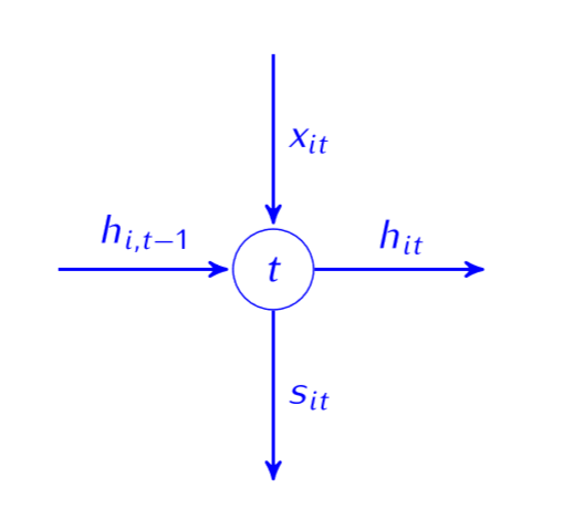
Define the three variables: Produced $x_{i t}$, sold $s_{i t}$ and held (stock) as $h_{it}$ $\forall i \in I, \ j \in J$.
Let $h_{i0}$ be the initial stock level (amount of held), we are given that there is nothing held as stock so $h_{i0} = 0, \forall i \in I$.
We need to have 50 units of each product at the end, so $h_{i6} = 50, \forall i \in I$.
The capacity bound the the held level is 100 units for each type, hence we impose the constraint: $h_{it}\le 100, \forall i\in I, \ \forall t\in T$.
We need to define a mass balance constraint, that ensures that last month stock plus this month produced is equal to this month stock plus this month sold. Written as:
$h_{i, t-1}+x_{it} = s_{it}+h_{it}, \qquad \forall i\in I, \forall t\in T$
Let the upper bound for the amount sold be denoted $u_{it}, \forall i\in I, \ \forall t\in T$.
The balance constraint can be view as:
Let $M = \{GR, VD, HD, BR, PL\}$ be the set of machines and let $c_j$ for $j\in M$ be the amnount of machines that the company has and let $m_{j,t}$ be the amount of machine $j\in M$ down for maintenance in month $t\in T$. Let $a_{ij}$ be the required input to produce product $i\in I$ of machine $j\in M$.
For each unit we held (place at stock) we pay the cost of 0.5 per unit of product per month. Let $p_i$ denote the profit for selling product $i\in I$. Our objective is maximizing profit minus storage cost. The model looks as follows:
$\begin{aligned} \text{max} & \qquad \sum\limits_{i\in I}\sum\limits_{t\in T}(p_is_{it}-0.5h_{it}) & \\ \text{s.t.} & \qquad \sum\limits_{i\in I}a_{ij}x_{it} \le 384(c_j-m_{jt}) & \forall j\in M, \ \forall t\in T \\ & \qquad h_{i, t-1}+x_{it} = s_{it}+h_{it} & \forall i\in I, \ \forall t\in T \\ & \qquad s_{it} \le u_{it} & \forall i\in I, \ \forall t\in T \\ & \qquad h_{it} \le 100 & \forall i\in I, \ \forall t\in T \\ & \qquad h_{i0}=0, \ h_{i6} = 50 & \forall i \in I \qquad \quad \space \\ & \qquad x_{it}, s_{it}, h_{it} \ge 0 & \forall i \in I, \ \forall t\in T \\ \end{aligned}$
The amount of variables is found by multiplying the three varibles by the amount of products and time periods.
print("Amount of variables:",3*6*7)
We can find the amount of constraints by counting each line of the model without including the non-negative constraints:
M = 5
T = 6
I = 7
print("Amount of constrains:",M*T+I*T+I*T+I*T+2*I)