DM560, Introduction to Programming in C++
Read the whole page before starting to work.
Graph Drawing
The following assignment is a shorter version of the one proposed by Ali Malik in his course Standard C++ Programming at Stanford University.
Graphs are mathematical structures used to model several real-life applications, for example, social networks, electric circuits, pipeline networks, lattices.
Task 1
In this task you are asked to write a program that defines:
-
a struct
nodecontaining the information on the name and the coordinates of a node; -
a struct
edgecontaining information on the tail (from node) and head (to node) of an edge; -
a class
Graphcontaining a vector ofnodeand a vector ofedge.
Make sure you can initialize, copy and print correctly the graph. In
particular overload the operator << to print the graph.
Finally, implement a reader that opens a given file and reads a graph in DIMACS format. Test your program on the following three graphs: marco10, line10, cube. Try to understand the encoding used and make sure that you can parse such files in a graph. Include all error checks described in Chapter 10. Print the graph read and make sure it is correct.
Task 2
Install the FLTK library and the interface
library Graph_lib. Try
to compile the program inside Graph_lib which implements the material
from chapter 12.
Draw the graph. Make up some coordinates for the points. For example,
place the points evenly spaced apart on the unit circle.
In
particular, in a graph with \(n\) nodes, node \(k\) should be placed at
\[
(\cos \frac{2\pi k}{n}, \sin \frac{2\pi k}{n} ).
\]
Here, angles are represented in radiants. In C++, you can compute sine
and cosine using the sin and cos functions exported by the <cmath>
header file. There is a predefined C++ constant for greek pi defined in
<cmath>, namely M_PI, but if it does not work in your system it
should be fine defining:
const double kPi = 3.14159265358979323;
Optional: modify your Graph Drawing program by including the enhancements implied by Exercises 1 to 6 of Chapter 13 on page 484. In particular, draw the graph with directed edges (ie, arcs). Make them curved. Draw nodes with their labels, and connection points on the border of the rectangle or circle that defines the nodes.
Task 3: Graph Layout Heuristics
In general, it can be difficult to find aesthetically pleasing layouts
for graphs. In this task, we investigate the question: given an
arbitrary graph, how can we produce a good drawing for that graph? This
is called the graph drawing problem and it has been studied
extensively. Interestingly, while there are many good algorithms for
drawing graphs, no one algorithm shines as ``the’’ graph drawing
algorithm. Every algorithm has its strengths and weaknesses, and many
algorithms that work marvelously on certain graphs will produce poor
layouts for other graphs. In this assignment, you’ll learn about one
particular type of algorithm called a force-directed layout algorithm
and will get a chance to see its performance on the three graphs listed
above. In doing so, you’ll work with the STL vector class and the FLTK
graphical library.
There are many heuristics that could be used to determine how good a graph drawing is. For example, we could try to minimize the number of arcs crossing one another, or try to maximize the symmetry of the drawing. In this assignment, however, we’ll limit ourselves to the following two heuristics, which work remarkably well in practice:
-
Position connected nodes near one another. When laying out a graph, it is often a good idea to place nodes that are joined by an edge near one another. The idea behind this metric is that if connected nodes are near each other, a reader can focus on one part of the graph and see the local structure of the graph in that region.
-
Maximize the distance between unconnected nodes. If two unconnected nodes are placed near one another, the reader can be confused into thinking that they are somehow related when in fact there is no connection between them.
In general, achieving these heuristics contemporaneously gives rise to a difficult problem. The position of each node influences the position of each other node, so picking a layout that balances the heuristics requires solving a large, complicated system of (nonlinear) equations. Fortunately, there is a clever strategy that lets us avoid this complexity.
Rather than searching for the answer directly, we’ll instead start off with a random guess, then continuously refine the positions of the nodes to improve upon the heuristics. Over time, the nodes will reach a position that balance the heuristics, and we’ll end up with an aesthetically pleasing graph drawing. The key step in this algorithm is finding some way to update the node positions, and to do this we’ll take a clue from physics. At each step of the graph layout, we’ll have the nodes exert forces on one another. These forces will push and pull nodes that are in suboptimal positions until they eventually come to rest in a stable location. Because we want unconnected nodes to be far apart from one another, we’ll have unconnected nodes repel each other node with some force. Similarly, because we want connected nodes to remain near one another, we’ll have each edge between nodes attract its endpoints. As these forces move the nodes around, the positions of the nodes will tend toward configurations where the net force on each node is minimized; that is, when there is a balance between the forces spacing out unconnected nodes and keeping together connected nodes.
The general skeleton of our algorithm is as follows:
Assign each node in the graph an initial location.
While the layout is not yet finished:
	Have each node exert a repulsive force on each other node.
	Have each edge exert an attractive force on its endpoints.
	Move the nodes according to the net force acting on them.
The details of each of these steps are quite customizable: we can initialize the positions of the nodes however we choose, decide when to stop based on multiple criteria, and use almost any function to determine the strengths of the attractive and repulsive forces between nodes. In this assignment, you’ll implement one particular version of a force-directed layout algorithm.
Assigning initial node positions. There is no one ``correct way’’ to initially lay out the nodes in the graph. Because the algorithm takes an initial guess and improves over time, pretty much any initial layout will do. In this assignment, however, you’ll initially position the nodes so that they are evenly spaced apart on the unit circle, as you have done earlier in Task 1.
Determining whether to continue iterating. The heart of the force-directed algorithm is the iteration. If the iteration cuts off too early, then the nodes may not have moved into good positions; if the iteration runs too long, then the computer will waste time trying to improve upon an already perfect layout. There are ways to decide when to terminate. A possibility is setting a time limit, alternatively it is possible to decide upon a position convergence. However, for simplicity we will terminate manually in this assignment.
Computing forces. The particular approach we will use to compute forces is based of of the Fruchterman-Reingold algorithm, an early but effective force-directed layout algorithm. In Fruchterman-Reingold, every node exerts a repulsive force on every other node that is inversely proportional to the distance between those nodes, and each arc exerts an attractive force on its endpoints proportional to the square of the distance between those nodes.
Only when the nodes are at a perfect distance from one another will the forces balance and the nodes cease to move.
To keep track of the net forces on each node, you’ll maintain a \(\Delta x\) and \(\Delta y\) value for each node which stores the net forces on that node along the \(x\) and \(y\) axes.
The first source of force acting on each node is the repulsive force exerted by every node against every other node. For each pair of nodes \( (x_0, y_0 ) \) and \( (x_1, y_1) \), their Euclidean distance is given by: \[ d=\sqrt{(x_1-x_0)^2+(y_1-y_0)^2} \] and the magnitude of the repulsive force \( F_{\mathrm{repel}} \) on the direction between the two nodes is \[ ||F_{\mathrm{repel}}|| = \frac{k_{\mathrm{repel}}}{d} \] where \( k_{\mathrm{repel}} \) is a constant that controls the strength of the repulsive attraction.
If the magnitude of this constant increases, then nodes repel each other more strongly; if it has a small magnitude, then nodes hardly repel each other at all.
The second source of force acting on each node is the attractive force between nodes joined together by edges. In this case, the magnitude of the attractive force \( F_{\mathrm{attract}} \) on the direction given by the two nodes is proportional to the square of the distance between the nodes:
\[ || F_{\mathrm{attract}} ||=\frac{ 1 }{\kappa_{\mathrm{attract}} } d^2=k_{\mathrm{attract}} \cdot d^2 \]
Again, \( k_{\mathrm{attract}} \) is a constant controlling the strength of the attractive force. As with \( k_{\mathrm{repel}} \) you will have to experiment with it. A good way is to test separately these two forces is by setting the constant of one of the two to zero and observing the effects. A possibly good starting guess is \( k_{\mathrm{repel}}=10^{3} \) and \( k_{\mathrm{attract}}=10^{-4} \) but you should experiment with other values.
Once you have computed the magnitude of these two opposite forces, you can determine for each of them how much is in the \( y \) direction and how much is in the \( x \) direction. To see how a force splits up, consider the following diagram:
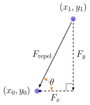
Here, \( F_x \) and \( F_y \) are the forces in the \( x \) and \( y \) directions exerted on the node \( (x_0, y_0) \). Using some simple trigonometry, we get that \[ F_{x0}=-F_{\mathrm{repel}} \cos \theta \] \[ F_{y0}=-F_{\mathrm{repel}} \sin \theta \] By Newton’s laws, the force exerted against the node \( (x1, y1) \) are thus \[ F_{x1}=F_{\mathrm{repel}} \cos\theta \] \[ F_{y1}=F_{\mathrm{repel}} \sin\theta \]
Here, we’ve been using the angle \( \theta \) to represent the angle indicated in the above drawing. Again, simple trigonometry tells us that
\[ \theta=\tan^{−1}\frac{y_1−y_0}{x_1−x_0} \]
Similar formulas can be written for the components of \( \vec{F}_{\mathrm{repel}} \) along the \( x \) and the \( y \) axis.
In C++, you can compute this arctangent using the atan2 function, also
in <cmath>. atan2 takes in two arguments - the first representing
\( y_1 - y_0 \) and the second \( x_1 - x_0 \) - and returns the
value of the above expression in radiants. For example:
double theta = atan2(y1 – y0, x1 – x0);
To summarize, the logic for computing all repulsive forces is as follows:
For each pair of nodes (x0, y0), (x_1, y1):
   Compute d = sqrt((y1 – y0)^2 + (x1 – x0)^2)
   Compute F_repel = k_repel / d
   Compute theta = atan2(y1 – y0, x1 – x0)
   Delta_x0 += Frepel cos(theta)
   Delta_y0 += Frepel sin(theta)
   Delta_x1 -= Frepel cos(theta)
   Delta_y1 -= Frepel sin(theta)
and for all attractive forces:
For each edge:
   Let the first endpoint be (x0, y0)
   Let the second endpoint be (x1, y1)
   Compute d = sqrt((y1 – y0)^2 + (x1 – x0)^2)
   Compute F_attract = k_attract * d^2
   Compute theta = atan2(y1 – y0, x1 – x0)
   Delta_x0 -= Fattract cos(theta) // Note that the sign here must be the opposite of above
   Delta_y0 -= Fattract sin(theta)
   Delta_x1 += Fattract cos(theta)
   Delta_y1 += Fattract sin(theta)
Moving Nodes According to the Forces. Once you’ve computed the net
Delta_x and Delta_y for each node, moving the nodes is an easy step
- simply increment each node’s
xcoordinate by itsDelta_xand each node’sycoordinate by itsDelta_y. Note that in a true physical simulation the forces on each object would change the velocity of the object rather than directly modifying its position, but for our simplified example changing position alone is sufficient. If you’d like to experiment with each node having a velocity and a position, feel free to do so.
The Assignment
Your assignment is to implement a simple program which reads in a graph from a file in DIMACS format (like the three given graphs), then runs the force-directed layout algorithm described above to find an appealing layout for the graph. In particular, your program should do the following:
-
Prompt the user for the name of a file containing the graph to visualize. Alternatively, if you are working in Linux you can get the name of the file from command line as an argument to the call of the program. For example:
graphviz marco10.dimacsthe argument can be taken in the
mainfunction of the C++ program modifying it as follows:int main (int argc, char **argv) { string inputfile; if (argc==2) { inputfile=argv[1]; } else { cout<<"graph filename"<<endl; exit(EXIT_FAILURE); } ... } -
Place each node into its initial configuration.
-
Iterate the following operations:
- Compute the net forces on each node.
- Move each node by the specified amount.
- Display the current state of the graph using the provided library.
You find a starter package Graphviz containing a framework where you have to insert your
code. In addition you will need the Graph_lib and the FLTK
libraries mentioned in Task 2.
The Package contains two empty files Graph.h and Graph.cpp for
the representation of the graph and the reader of a graph from a
file. You should have these methods from Task 1.
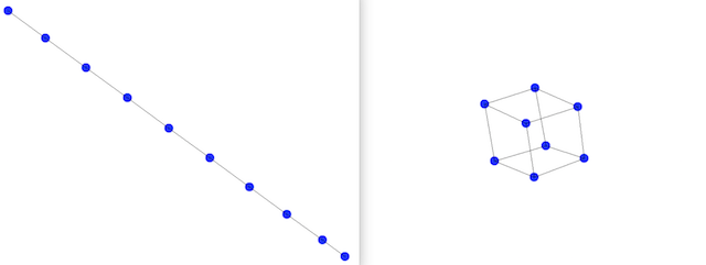
The package contains also sample graphs to test your program. The file
cube.dimacs contains a graph whose vertices represent the corner of a
cube and the graph line10.dimacs a line graph.
The animation can be created by redrawing the graph at every frame. The function
Fl::add_timeout(1, call_back, &g);
from the FLTK library adds a one-shot timeout callback to the function
call_back with an optional argument for this function. The function will be
called by Fl::run() at 1 second after Fl::run() is called. The
optional third argument is of type void∗ and is an argument to be
passed to the callback.
In the call_back function
Fl::repeat_timeout(1/48.0,call_back,graph);
repeats the timeout callback from the expiration of the previous timeout.
Task Breakdown
Although this topic is fairly lengthy, don’t panic - you don’t need to write very much code to complete this assignment.
-
Develop your code to represent and read the graph (we have done this also during the course). Start with small tasks, for example printing the name of the file, then printing the number of nodes and finally printing the edges. Use an internal index starting from 0 to represent the nodes, the graphs in the files have nodes labels starting from 1.
-
Implement the logic to initially position the nodes in the
mainfunction. Before you can run the force-directed algorithm, you will need to position all of the nodes in the graph in a circle. Test this step. -
Implement the force-directed layout algorithm in the
call_backfunction. This is the core of the assignment, but fortunately the code necessary to get it working is not too daunting. As a test of whether your code is working, if you run the algorithm on the graphline10, your algorithm should eventually end up arranging the points in a straight line. Similarly, running the algorithm on the filecubeshould arrange the points in a way that looks like a 3D perspective drawing of a cube.
Possible Extensions
This is a list of extensions within reach with just a of few lines more of code.
-
Experiment with different values for the two parameters in the forces.
-
Consider the frame and avoid vertices skipping out. For example remove a force if it makes a vertex go out of the frame.
-
Add random perturbations when the configuration is converged
-
Add node accelerations and velocities. This requires memorizing the movements in the previous iteration.