Online compendium to the article: |
In Ed. P. Festa, Proceedings of the 9th International Symposium on Experimental Algorithms 2010,
Lecture Notes in Computer Science, Springer
Tot. Size Type Density Variability Hidden colouring graphs 500 G 0.1 0 5 10 10 | | | 1 5 10 10 | | | no – 10 | | 0.5 0 20 30 40 50 60 25 | | | 1 20 30 40 50 60 25 | | | no – 10 | | 0.9 0 20 30 40 60 80 100 120 140 40 | | | 1 20 30 40 60 80 100 120 140 40 | | | no – 10 | U 0.1 0 10 20 10 | | | 1 10 20 10 | | | no – 10 | | 0.5 0 20 30 40 50 60 70 80 90 100 110 50 | | | 1 20 30 40 50 60 70 80 90 100 110 50 | | | no – 10 | | 0.9 0 100 150 200 250 300 25 | | | 1 100 150 200 250 300 25 | | | no – 10 | W 0.1 0 5 10 10 | | | 1 5 10 10 | | | no – 10 | | 0.5 0 20 30 40 50 60 25 | | | 1 20 30 40 50 60 25 | | | no – 10 | | 0.9 0 30 60 90 120 20 | | | 1 30 60 90 120 20 | | | no – 10 1000 G 0.1 0 5 10 20 15 | | | 1 5 10 20 15 | | | no – 10 | | 0.5 0 20 30 40 50 60 70 80 90 100 110 120 130 140 75 | | | 1 20 30 40 50 60 70 80 90 100 110 120 130 140 75 | | | no – 10 | | 0.9 0 20 50 100 150 200 250 30 | | | 1 20 50 100 150 200 250 30 | | | no – 10 | U 0.1 0 20 30 40 50 20 | | | 1 20 30 40 50 20 | | | no – 10 | | 0.5 0 20 30 40 50 60 70 80 90 100 110 120 130 140 150 160 170 180 190 200 95 | | | 1 20 30 40 50 60 70 80 90 100 110 120 130 140 150 160 170 180 190 200 95 | | | no – 10 | | 0.9 0 100 200 300 400 500 600 30 | | | 1 100 200 300 400 500 600 30 | | | no – 10 | W 0.1 0 10 20 10 | | | 1 10 20 10 | | | no – 10 | | 0.5 0 20 30 40 50 60 70 80 90 40 | | | 1 20 30 40 50 60 70 80 90 40 | | | no – 10 | | 0.9 0 30 90 150 220 20 | | | 1 30 90 150 220 20 | | | no – 10
Table 1: The table shows how the 1260 graphs generated are distributed over the features. The number of graphs of size 500 is 520 and those of size 1000 is 740.
The computation time that TSN1 needs to perform Imax iterations varies due to several factors.
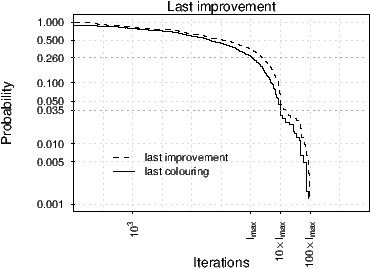
In Figure 1 left, we plot the probability of finding a feasible colouring and an improvement in solution quality (i.e., a decrease in the number of colour conflicts) after a certain number of iterations. The graph is obtained by recording the last corresponding events occurred in a run of TSN1 on each of the 740 random graphs of size 1000. TSN1 was run on all graphs for a maximum number of 100 × Imax iterations. The curves correspond to the empirical survival distributions of the event “finding a colouring with less constraint violations” or “finding a feasible colouring”. In other words, each point indicates the probability of finding a graph where improvements in the number of constraint violations or in the number of colours can still occur after a certain number of iterations, reported on the x-axis.
Both types of improvements after 50 × Imax iterations occurred only in 10 graphs, that is, with a probability lower than 0.02. The number of colouring violations in these extreme cases was below 13 and, we should not discard the possibility that further improvements could have been possible with longer runs. Therefore, these data should be treated as censored data and the curve be truncated. Nevertheless, for 730 of the 740 graphs no further improvement in the solution occurred in the last 50 × Imax iterations, which lets us conjecture that further improvements will not occur on those graphs. However, the plot also indicates, that after Imax iterations a feasible colouring was still found for 26% of the graphs. In other terms, setting the termination criterion to Imax corresponds to miss 26% of cases where a better colouring can still be found. This empirical probability falls below 3% after 10 × Imax. The probability of finding improvements in solution quality is slightly higher, 35% after Imax and 5% after 10 × Imax.
In the light of these results, 10 × Imax would have been a better choice for the termination criterion of TSN1. However, 10 × Imax corresponds on average, to an increase in computation time of a factor of 10 with respect to Imax and we could not afford this cost in our computational environment. Therefore, we decided to use Imax.
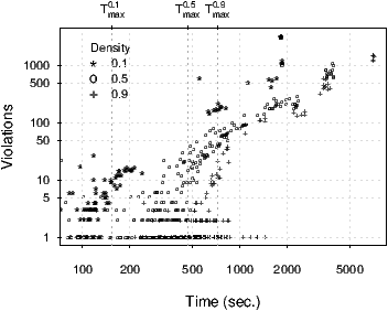
In Figure 1, right, we investigate the computation time corresponding to Imax iterations on graphs of 1000 vertices. Clearly, the reason for uncommonly long run times for TSN1 to perform Imax iterations is a high number of violations in the solutions since the neighbourhood size of N1 is dynamically linked to the number of colours and the number of vertices involved in at least one colour conflict. The plot shows the correlation between the number of violations present in the final solution and the time elapsed between the time-point when a last feasible colouring is found and when the maximal number of iterations is passed. Evidently, long run times arise in cases where a lot of time is spent for numbers of colours that cause many violations. Very likely, in those cases there exists no better feasible colourings and the run could be aborted. The run time limits of Table 1(d) in the paper, that correspond to median values per edge density, appear, therefore, plausible because they cut out those useless long run times. On the other hand, run times of around 150, 700, and 1500 seconds for graphs of density, respectively, 0.1, 0.5, 0.9 are enough for TSN1 to accomplish Imax iterations on the graphs with only few violations, that is, for those situations where it is reasonable to use all the iterations available. Note that the time limit adopted for graphs of density 0.9 appears underestimated and could be the reason for some of those feasible colouring missed in the interval [Imax,10 × Imax] of Figure 1, left.
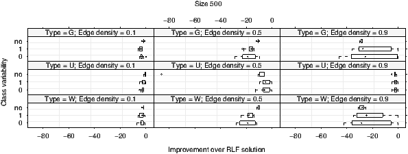
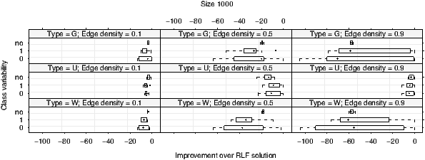
The use of SLS heuristics gives a significant improvement over the initial solution of RLF. In Figure 2, we show the distribution of differences between the best solutions found in a graph by the SLS heuristics and the initial RLF solution. We distinguish two main patterns which have an impact on the entity of the improvement. First, the improvement increases considerably with size and edge density for Uniform and Weight Biased graphs and it can reach 105 colours of improvement in the case of Weight Biased graphs. Second, in Geometric graphs, the improvement is smaller than for the other two types of graphs and more pronounced in graphs of density 0.5. These results on the Geometric graphs together with the results of Ex-DSATUR on those graphs let us conclude that on these graphs RLF finds already a near-optimal solution.